Sit with people that ARE NOT in your project group.
Recap
ImportantStatistical superpowers
In practice, we often have specific hypotheses about the population of interest. We can test these hypotheses using our sample data!!
NoteLearning goals
By the end of this lesson, you should be able to:
Understand how standard errors and confidence intervals enable us to make statistical inferences
Articulate how we can formalize a research question as a testable, statistical hypothesis
NoteAdditional resources
This is a discovery activity, so no readings/videos today.
Warm-up
Let’s return to the fish dataset. Recall that rivers contain small concentrations of mercury which can accumulate in fish. Scientists studied this phenomenon among 171 largemouth bass in the Wacamaw and Lumber rivers of North Carolina, recording the following:
variable
meaning
River
Lumber or Wacamaw
Station
Station number where the fish was caught (0, 1, …, 15)
Length
Fish’s length (in centimeters)
Weight
Fish’s weight (in grams)
Concen
Fish’s mercury concentration (in parts per million; ppm)
# Load the data & packageslibrary(tidyverse)fish <-read_csv("https://mac-stat.github.io/data/Mercury.csv")head(fish)
Use this sample data to make inferences about the relationship of mercury concentration (Concen) with the size of a fish, as measured by its Length. This relationship can be described by the population model:
fish_mod_1 <-lm(Concen ~ Length, data = fish)summary(fish_mod_1)
Call:
lm(formula = Concen ~ Length, data = fish)

Residuals:
    Min      1Q  Median      3Q     Max
-1.1499 -0.3436 -0.1022  0.3123  1.9100

Coefficients:
             Estimate Std. Error t value Pr(>|t|)
(Intercept) -1.131645   0.213615  -5.298 3.62e-07 ***
Length       0.058127   0.005228  11.119  < 2e-16 ***
---
Signif. codes:  0 '***' 0.001 '**' 0.01 '*' 0.05 '.' 0.1 ' ' 1

Residual standard error: 0.5805 on 169 degrees of freedom
Multiple R-squared:  0.4225,    Adjusted R-squared:  0.4191
F-statistic: 123.6 on 1 and 169 DF,  p-value: < 2.2e-16
Example 1: Review
Notation:
\beta_1 = the population parameter of interest whose “true” value is unknown
\hat{\beta}_1 = 0.058 is our sample estimate of \beta_1
SE(\hat{\beta}_1) = 0.005 is the standard error of \hat{\beta}_1
Interpret \hat{\beta}_1.
Using the 68-95-99.7 rule, construct an approximate 95% confidence interval for \beta_1. That is, calculate an interval estimate of \beta_1.
Compare your CI to an exact 95% CI:
___(___, level =0.95)
Interpret the 95% CI in context.
Example 2: Translating a hypothesis to notation
Our work above provides point and interval estimates of \beta_1. But we also want to test hypotheses related to \beta_1.
Our fundamental hypothesis here is that, among the fish population, mercury levels are associated with fish length – there’s a relationship between the two.
How can we state this hypothesis using notation? Choose 1.
\beta_1 = 0
\beta_1 \ne 0
\hat{\beta}_1 = 0
\hat{\beta}_1 \ne 0
\beta_0 = 0
\beta_0 \ne 0
\hat{\beta}_0 = 0
\hat{\beta}_0 \ne 0
NOTE: We’ll refer to 0 as the null value to which we’re comparing our population parameter of interest.
Example 3: Evaluating a hypothesis using the CI
Since we don’t have access to the entire fish population, we must evaluate our hypothesis using our sample data. We have to ask: does our sample data provide enough evidence to support the hypothesis that, among the fish population, not just our sample, mercury levels are associated with fish length?
Explain why we can’t use our simple estimate \hat{\beta}_1 to evaluate this hypothesis, but we can use the 95% CI for \beta_1. (This is true in general, not just this fish example!)
So, does your 95% CI from Example 1 support the hypothesis that there’s a relationship between mercury levels and fish length? Explain.
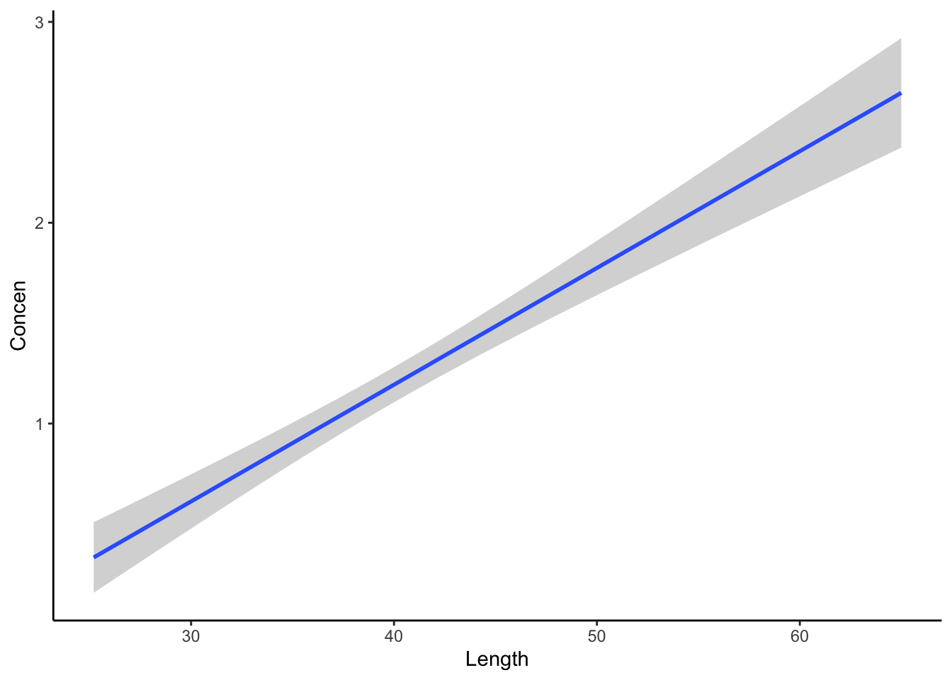
Similarly, do the confidence bands below support the hypothesis?
fish %>%ggplot(aes(y = Concen, x = Length)) +geom_smooth(method ="lm")
FORMAL HYPOTHESIS TESTS
Though CIs can help us evaluate hypotheses, hypothesis tests provide a more formal approach. The general idea:
Assume that the hypothesis is not true.
Determine what sample observations would be expected under this assumption.
Evaluate how compatible our observed sample data are with this assumption (are they consistent with what we’d expect?).
Or, in context:
Assume there were truly no association between mercury concentration and fish length, i.e. \beta_1 = 0 (the “null value”).
Determine how our fish sample might have “behaved” if there were truly no association.
Evaluate how compatible our fish sample observations are with the null value (are they consistent with what we’d expect if there were no association?).
Exercises
NOTE
The goal of these exercises is to explore concepts in hypothesis testing. There’s some new code that helps with this exploration, but the code is not the point!! Throughout, focus on the goal of the code and what its output tells us, NOT the details of the code.
Our results will start to use more scientific notation. Examples:
3e-02 = 0.03 (move the decimal 2 places to the left)
3e02 = 300 (move the decimal 2 places to the right)
4.12e-07 = 0.000000412 (move the decimal 7 places to the left)
4.12e03 = 4120 (move the decimal 3 places to the right)
< 2e-16 = the result is less than 0.0000000000000002 (it’s really really small!)
Exercise 1: Simulating data under the null value
To begin testing our hypothesis that there is an association between mercury concentration and fish length (\beta_1 \ne 0), let’s explore how our sample data might behave IF in fact there were no association (\beta_1 = 0). We’ll first do this using simulation, and then through theory.
Read carefully:
Suppose that when each individual fish in our sample was collected, the scientists wrote its Concen and Length on a piece of paper.
They then ripped the paper in half, with the observed Concen on one half and the observed Length on the other.
They then accidentally dropped the pieces of paper! In the resulting mess, they couldn’t tell which Length observation went with each Concen observation.
To cover up their mistake, they just randomly matched up the Length and Concen pieces of paper. Essentially, in this shuffling process, the scientists broke the bond of the original Length and Concen pairs.
Question: Intuitively, if the researchers plotted the new pairs of Concen and Length values, what do you think their scatterplot would look like? What about their sample model?
We can simulate this idea in RStudio! Throughout, focus on concepts over code.
# First check out the first 6 fishfish %>%select(Concen, Length) %>%head()
Now, randomly shuffle the Length values! That is, break the original Concen and Length pairs, and just randomly assign Length:
# Run this chunk a few times!!# Shuffle the Length valuesfish %>%select(Concen, Length) %>%mutate(Length =sample(Length, size =length(Length), replace =FALSE)) %>%head()
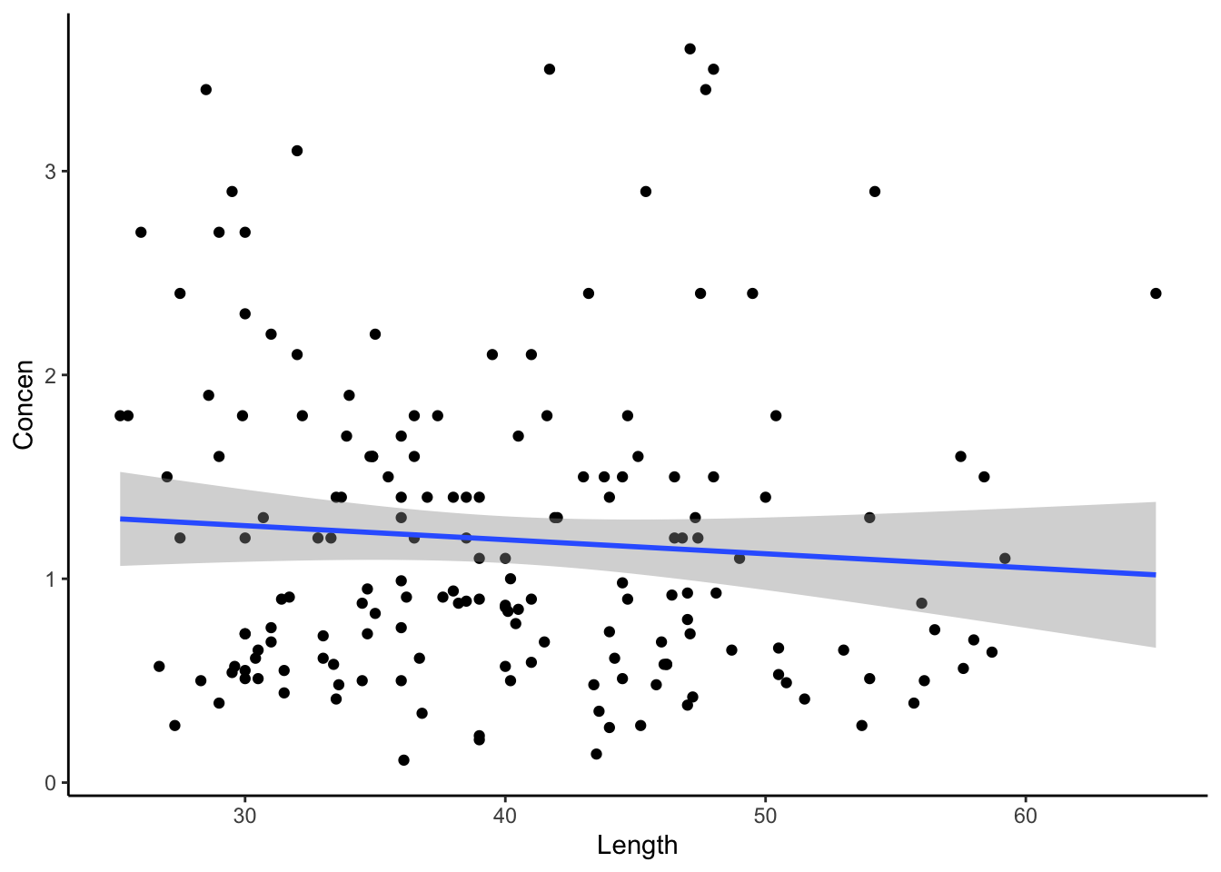
Let’s check out the sample models that arise from the shuffled Concen and Length pairs. Summarize your observations! Was your intuition in Part a correct?
# Shuffle the Length values# Run this chunk a few times!!# Then plot the resulting sample data and modelfish %>%select(Concen, Length) %>%mutate(Length =sample(Length, size =length(Length), replace =FALSE)) %>%ggplot(aes(x = Length, y = Concen)) +geom_point() +geom_smooth(method ="lm")
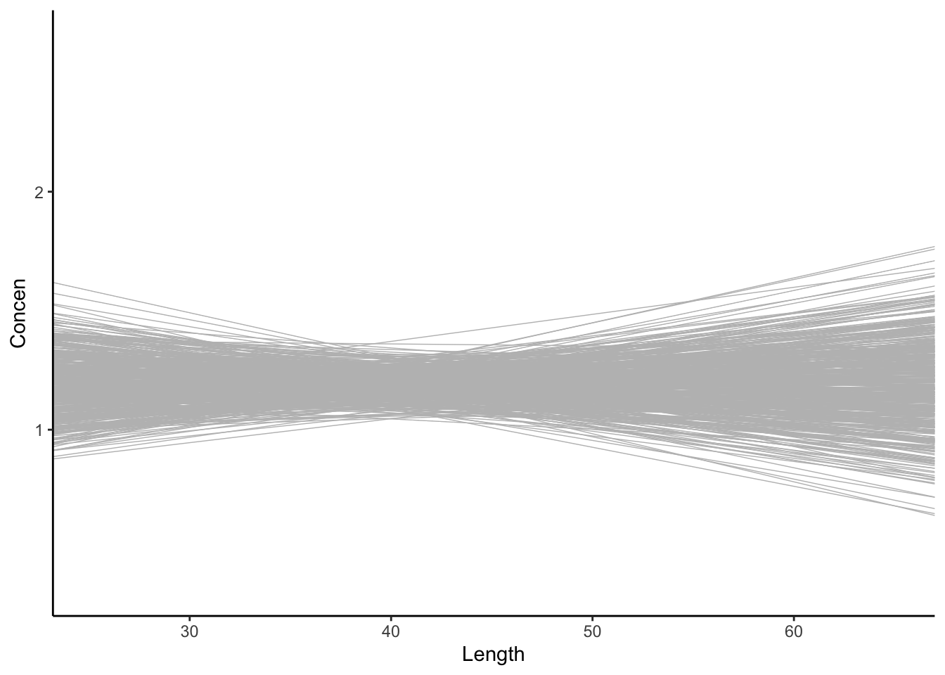
These shuffled samples give us a sense of the sample models we’d expect IF \beta_1 were actually 0, i.e. if there were no relationship between Concen and Length in the broader population of fish. To get a sense of the range of possible outcomes in this scenario, let’s simulate a bunch of shuffled samples. Specifically, take 500 different shuffled samples and use each to estimate the model of Concen by Length (gray lines). Summarize your observations!! If there were truly no relationship between Concen and Length, how would we expect the sample data to behave?
# Plot the 500 shuffled modelsfish %>%ggplot(aes(x = Length, y = Concen)) +geom_abline(data = shuffled_models, aes(intercept =`(Intercept)`, slope = Length), color ="gray", size =0.25) +geom_smooth(method ="lm", se =FALSE, size =0) # Ignore this line. It's a clunky workaround
Finally, focus on just the slope estimates \hat{\beta}_1 behind the lines above. Summarize your observations!! If there were truly no relationship between Concen and Length, i.e. \beta_1 were truly 0, how would we expect the sample slopes to behave?
Exercise 2: Comparing our sample results to the null value (intuition)
Now that we’ve simulated how sample data might behave if there were truly no relationship between Concen and Length (i.e. if \beta_1 were 0), let’s consider the next important step in a hypothesis test:
Evaluate how compatible our observed sample data are with this assumption that \beta_1 = 0!
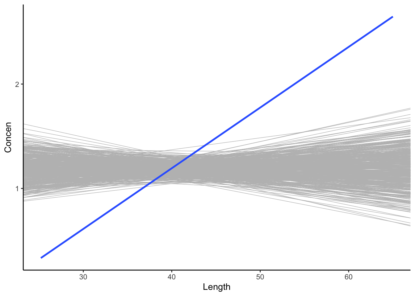
Let’s start with a visual assessment. Is our sample model (blue line) consistent / compatible with the “null models” simulated under the assumption the \beta_1 = 0 (gray lines)?
fish %>%ggplot(aes(x = Length, y = Concen)) +geom_abline(data = shuffled_models, aes(intercept =`(Intercept)`, slope = Length), color ="gray", size =0.25) +geom_smooth(method ="lm", se =FALSE)
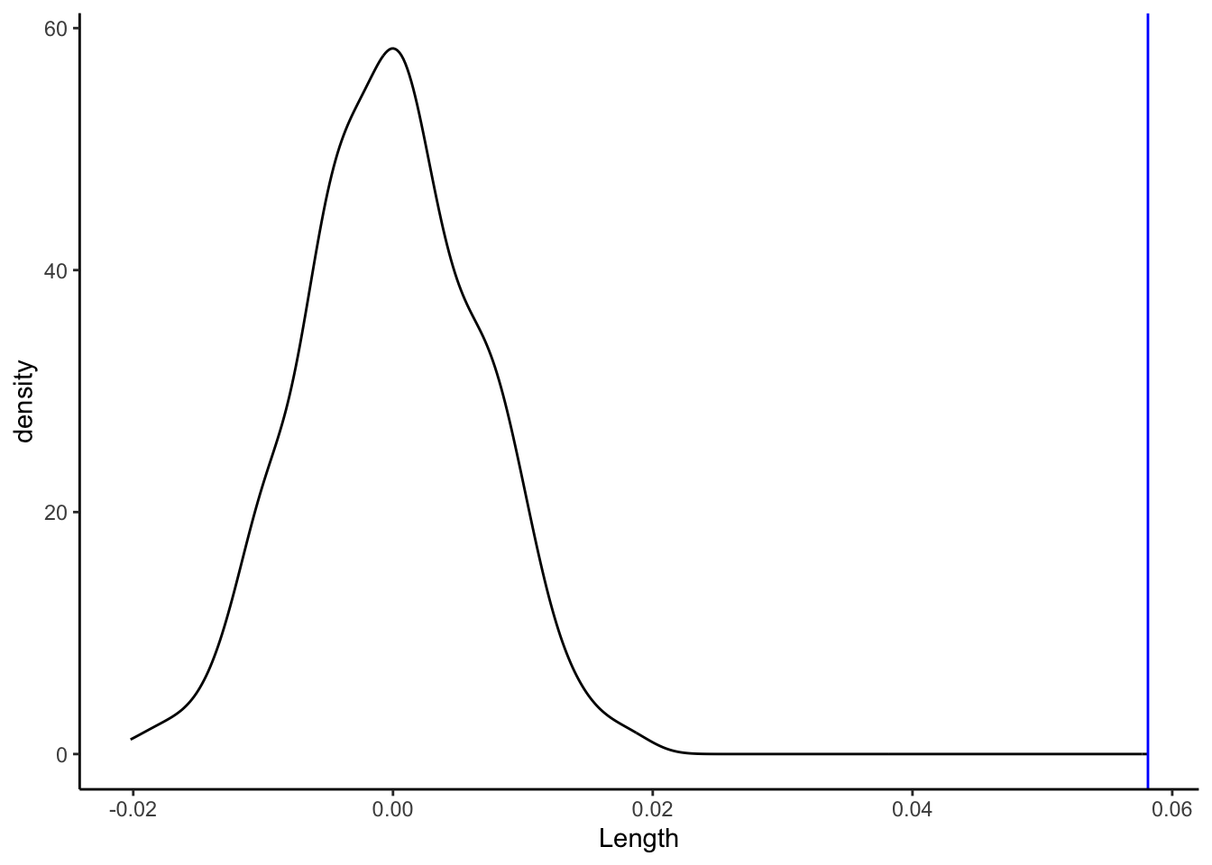
Consider another visual assessment, focusing just on the slopes of the lines in the plot above, i.e. our sample estimates \hat{\beta}_1. Is our sample slope of \hat{\beta}_1 = 0.05813 (blue line) consistent / compatible with the collection of slopes from the “null models” (density plot)?
shuffled_models %>%ggplot(aes(x = Length)) +geom_density() +geom_vline(xintercept =0.05813, color ="blue")
In Part b, you evaluated the compatibility of our sample slope \hat{\beta}_1 = 0.05813 model with slopes of the “null models” using visual cues alone. But for a formal hypothesis test, we need some numerical measures of compatibility. Brainstorm some ideas!
Exercise 3: CLT
Now that we’ve built up some intuition using simulation, let’s formalize these concepts with some theory.
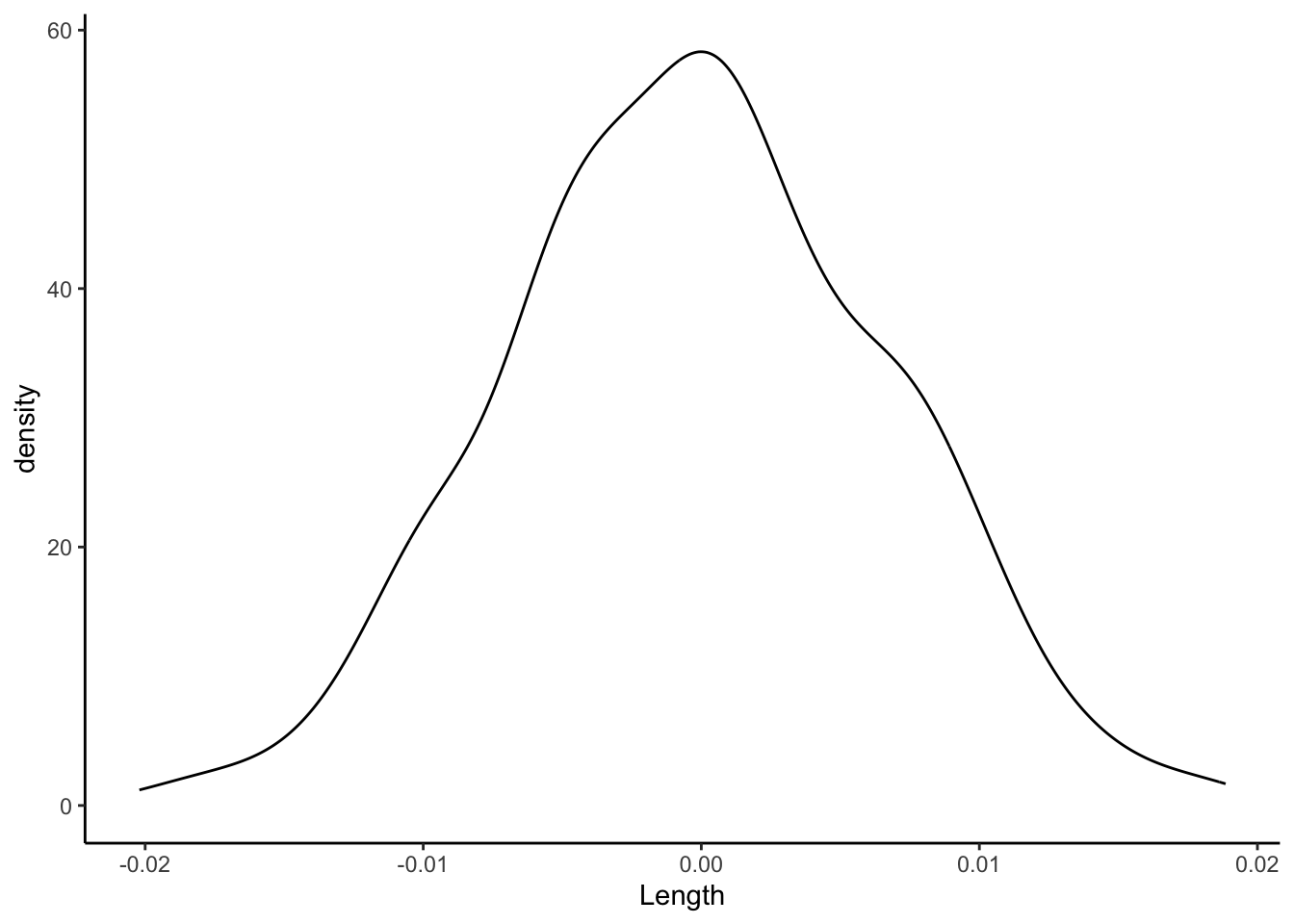
You shouldn’t be surprised to know that sampling distributions are at the heart of hypothesis testing! The distribution of slopes from our shuffled sample models uses simulation to approximate the sampling distribution of slope estimates \hat{\beta}_1 we’d expect if the population slope \beta_1 were actually 0 (the null value):
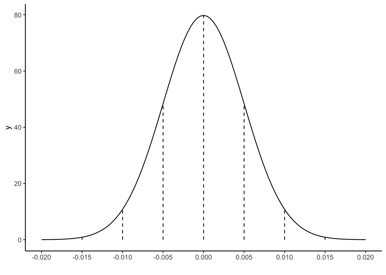
We can also approximate the sampling distribution using mathematical theory, specifically the Central Limit Theorem. If \beta_1 were truly 0, then the distribution of possible sample estimates \hat{\beta}_1 would be Normally distributed around 0:
\hat{\beta}_1 \sim N(0, SE(\hat{\beta}_1)^2)
where in Example 1 we approximated the standard error to be 0.005. Thus a plot of the CLT is below. Confirm that this is similar to the simulated sampling distribution above:
# Don't worry about this code!!!# Save your plotclt_plot <-data.frame(x =0+c(-4:4)*0.005) %>%mutate(y =dnorm(x, sd =0.005)) %>%ggplot(aes(x = x)) +stat_function(fun = dnorm, args =list(mean =0, sd =0.005)) +geom_segment(aes(x = x, xend = x, y =0, yend = y), linetype ="dashed") +scale_x_continuous(breaks =c(-4:4)*0.005) +xlab("")clt_plot
Exercise 4: Comparing our sample results to the null value (test statistic)
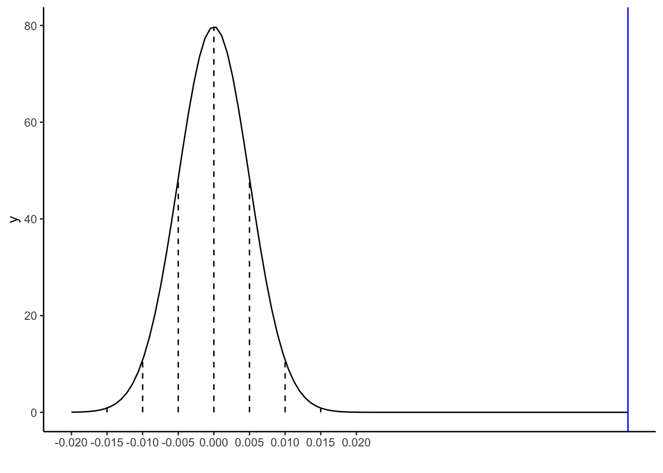
Our sample slope estimate of \hat{\beta}_1 = 0.05813 is shown on the sampling distribution of sample slopes \hat{\beta}_1 that we’d expect if the population slope \beta_1 were actually 0 (the null value):
clt_plot +geom_vline(xintercept =0.05813, color ="blue")
To measure how compatible (or incompatible) our estimate is with the null value, we can measure the distance between the two.
Our sample slope estimate of \hat{\beta}_1 = 0.05813 is 0.05813 units (ppm/cm) from the null value of 0.
In the context of this particular analysis, is that a big or a small number? How can you tell? That is, what info are you using to make this assessment?
Would your answer be the same if you observed this estimate in another context?
In practice, we standardize our distance calculations so that they have the same meaning no matter the context of the analysis. We can do this by calculating a z-score:
\frac{\hat{\beta}_1 - \text{null value}}{SE(\hat{\beta}_1))} = \text{ number of SE that $\hat{\beta}_1$ falls from the null value}
This is called the test statistic. Calculate and interpret the test statistic for our example.
Within rounding, the same test statistic appears in our model summary table! Where is it?!
coef(summary(fish_mod_1))
What can we conclude from your test statistic calculation and interpretation:
Our sample data is not consistent with the null value of \beta_1 = 0, i.e. the idea that there’s no significant association between mercury concentration and length.
Our sample data is consistent with the null value of \beta_1 = 0.
Exercise 5: Comparing our sample results to the null value (p-value)
Again, our sample slope estimate of \hat{\beta}_1 = 0.05813 is shown on the sampling distribution of sample slopes \hat{\beta}_1 that we’d expect if the population slope \beta_1 were actually 0 (the null value):
clt_plot +geom_vline(xintercept =0.05813, color ="blue")
Another way to evaluate the compatibility of our estimate with the null value of \beta_1 = 0 is to ask how likely we are to have gotten this estimate if the null value were indeed true! That is, what’s the probability that we would have gotten a sample slope that’s at least 0.058 above or below 0 IF in fact there were no association between mercury concentration and length? Equivalently, what’s the probability that we would have gotten a test statistic so far from 0 IF in fact \beta_1 were 0?
Use the 68-95-99.7 Rule with the plot above to approximate the p-value:
less than 0.003
between 0.003 and 0.05
between 0.05 and 0.32
bigger than 0.32
The calculation above is called a p-value. A more accurate p-value is reported in the model summary table in the Pr(>|t|) column. What is it?
coef(summary(fish_mod_1))
How can we interpret the p-value? IMPORTANT: Think about the steps that went into calculating the p-value!!
It’s very unlikely that we’d have observed such a steep increase in Concen with Length among our sample fish “by chance”, i.e. if in fact there were no relationship between mercury concentration and length in the broader fish population.
Given what we observed in our sample data, it’s very unlikely that mercury concentration is associated with length.
Given what we observed in our sample data, it’s very unlikely that mercury concentration and length are unrelated.
PAUSE: Check the solutions to this question! p-values are commonly misinterpreted.
Exercise 6: River test Part I
The fish in our sample come from two different rivers: Lumber and Wacamaw. Research question: Is there evidence that the mercury concentration in fish differs between the 2 rivers?
To answer this question, we’ll control for fish Length – we don’t want to mistakenly detect a difference in mercury levels just because we happened to sample bigger fish in one river and smaller fish in the other. The relevant population model is:
To address the above research question, which model coefficient / population parameter is of primary interest: \beta_0, \beta_1, or \beta_2? And what’s the null value of this coefficient? That is, what would this coefficient be if there were truly no difference in mercury concentration between the 2 rivers (when controlling for length)?
For the parameter of interest, obtain and report a sample estimate and its corresponding standard error:
fish_mod_2 <-lm(___, data = fish)coef(summary(fish_mod_2))
Let’s use this data to evaluate our research question. To do so, remember the next step: Assume that the null value from Part a is correct and determine what sample estimates we would expect to get in this scenario.
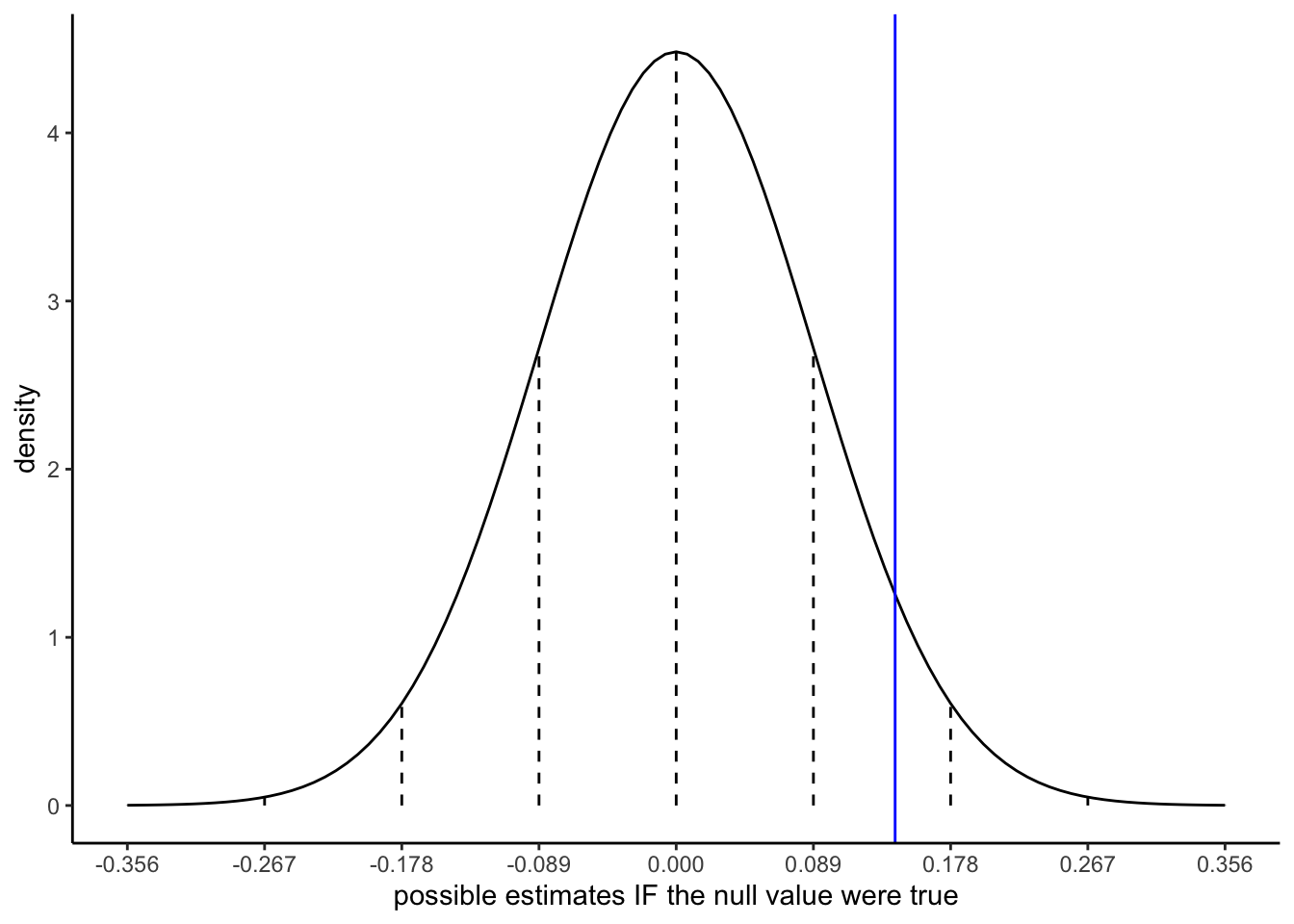
Adjust the code below to sketch the appropriate sampling distribution. Represent our sample estimate by a blue line.
# Put OUR sample estimate here# Round to 3 digitsest <- ___# Put the corresponding standard error here# Round to 3 digitsse <- ___data.frame(x =0+c(-4:4)*se) %>%mutate(y =dnorm(x, sd = se)) %>%ggplot(aes(x = x)) +stat_function(fun = dnorm, args =list(mean =0, sd = se)) +geom_segment(aes(x = x, xend = x, y =0, yend = y), linetype ="dashed") +scale_x_continuous(breaks =c(-4:4)*se) +geom_vline(xintercept = est, color ="blue") +labs(y ="density", x ="possible estimates IF the null value were true")
Exercise 7: River test Part II
Remember the next step: We must evaluate how compatible our sample estimate is with the null value. We’ll take 3 approaches: using a visual assessment, test statistic, and p-value.
Visually, in Part c of the previous exercise, does our sample estimate seem compatible with the null value? Mainly, is our estimate consistent with what we’d expect to observe if there were truly no difference in the mercury concentration between the 2 rivers (when controlling for fish length)?
Let’s focus on the test statistic:
Obtain the test statistic from the model summary table below.
Show how this was calculated from the sample estimate and its standard error.
Interpret the test statistic.
coef(summary(fish_mod_2))
Recall that the p-value calculates the probability that, IF in fact the null value were correct (i.e. there was actually no difference in mercury concentration by river when controlling for length), we would have gotten a sample estimate that’s as far from the null value as ours, either above or below.
Use the 68-95-99.7 Rule with the plot in Part c of the previous exercise to approximate the p-value:
less than 0.003
between 0.003 and 0.05
between 0.05 and 0.32
bigger than 0.32
Now obtain and report the exact p-value from the model summary table.
Do your test statistic and p-value indicate that your estimate is or is not compatible with the null value? Explain.
Putting this all together, what do you conclude? When controlling for length…
we have evidence of a statistically significant difference in mercury concentration by river.
we do not have sufficient evidence to conclude that there’s a statistically significant difference in mercury concentration by river.
Exercise 8: River CI
Finally, construct a 95% CI for the population parameter of interest in our river analysis.
What do you conclude from this CI? When controlling for length…
we have evidence of a statistically significant difference in mercury concentration by river.
we do not have sufficient evidence to conclude that there’s a statistically significant difference in mercury concentration by river.
Your conclusions from the hypothesis test (test statistic and p-value) should agree with those from your CI! If this is not the case, review your work.
Wrap-up
Finish and study the activity!
PS 6 due tonight
Check out the course schedule for other upcoming due dates.
Reminders:
Remember the important basics: complete activities, ask for help, study on a regular basis, start assignments early.
If you miss class on a project day, it’s your responsibility to communicate with your group, find out what you missed, and make equivalent contributions outside of class. If missing class on project days becomes a pattern, it will impact your project grade.
Your final project grade will reflect your individual engagement and contributions to the project. You are not expected to be perfect. Rather, you should put effort, attention, and reflection into the following areas:
communication
contributing to group discussions
including all other group members in discussion
creating a space where others felt comfortable sharing ideas and mistakes
communicating with your group outside class
report contributions
contributing to the content / analysis in the report
contributing to the writing of the report
contributing to the editing of the report
Solutions
Warm Up
# Load the data & packageslibrary(tidyverse)fish <-read_csv("https://mac-stat.github.io/data/Mercury.csv")head(fish)
# Run this chunk a few times!!# Shuffle the Length valuesfish %>%select(Concen, Length) %>%mutate(Length =sample(Length, size =length(Length), replace =FALSE)) %>%head()
# Shuffle the Length values# Run this chunk a few times!!# Then plot the resulting sample data and modelfish %>%select(Concen, Length) %>%mutate(Length =sample(Length, size =length(Length), replace =FALSE)) %>%ggplot(aes(x = Length, y = Concen)) +geom_point() +geom_smooth(method ="lm")
If there were truly no relationship between Concen and Length, we’d expect the sample model to have a slope near to (but not exactly) 0.
Exercise 4: Comparing our sample results to the null value (test statistic)
Solution
clt_plot +geom_vline(xintercept =0.05813, color ="blue")
How far is our sample slope estimate of \hat{\beta}_1 = 0.05813 from the null value of 0? 0.05813 :)
In the context of this particular analysis, is that a big or a small number? How can you tell? This seems pretty big relative to the standard error.
Our sample slope of 0.058 falls more than 11 standard errors above the null value of 0. That’s far!!!
(0.058127-0) /0.005228
[1] 11.1184
In the t value column:
coef(summary(fish_mod_1))
               Estimate  Std. Error   t value     Pr(>|t|)
(Intercept) -1.13164542 0.213614796 -5.297598 3.617750e-07
Length       0.05812749 0.005227593 11.119359 6.641225e-22
Our sample data is not consistent with the null value of \beta_1 = 0, i.e. the idea that there’s no significant association between mercury concentration and length.
Exercise 5: Comparing our sample results to the null value (p-value)
Solution
clt_plot +geom_vline(xintercept =0.05813, color ="blue")
Our estimate is more than 3 SE away from 0. Since 99.7% of estimates fall within 3 SE the probability of this happening is…
less than 0.003 (1 - 0.997)
< 2e-16 (which is very very close to 0)
coef(summary(fish_mod_1))
               Estimate  Std. Error   t value     Pr(>|t|)
(Intercept) -1.13164542 0.213614796 -5.297598 3.617750e-07
Length       0.05812749 0.005227593 11.119359 6.641225e-22
It’s very unlikely that we’d have observed such a steep increase in Concen with Length among our sample fish “by chance”, i.e. if in fact there were no relationship between mercury concentration and length in the broader fish population.
Exercise 6: River test Part I
Solution
\beta_1, the RiverWacamaw coefficient
The null value is \beta_1 = 0
\hat{\beta}_1 = 0.142 with a standard error of 0.089:
fish_mod_2 <-lm(Concen ~ River + Length, data = fish)coef(summary(fish_mod_2))