21 Confidence intervals

Settling In

Today will be a no computer day!
After class, you can find the qmd with code and extra exercises here: “21-confidence-intervals-notes.qmd”.

Recap

Statistical superpowers

When using our sample data to make estimates about the population, we can do better than providing a single best guess. We can obtain a range of guesses that better captures our understanding and reflects the potential error in our estimate. This is a confidence interval.

Learning goals

By the end of this lesson, you should be able to:

Construct (approximate) confidence intervals by hand using the 68-95-99.7 rule
Construct exact confidence intervals in R
Interpret confidence intervals in context by referring to the coefficient of interest
Use confidence intervals to make statements about whether there appear to be true population relationships, changes, and differences

Additional resources

Required:

Video : Introduction to Confidence Intervals
Reading: Section 7 Introduction, Section 7.1, Section 7.2 (stop when you get to 7.2.4.3 Confidence Intervals for Prediction) in the STAT 155 Notes

Optional:

Video 2: Confidence Intervals: Construction and Interpretation

Confidence Intervals

Set-up

\beta = some population parameter (e.g. a model coefficient)
\hat{\beta} = a sample estimate of \beta
\text{SE}(\hat{\beta}) = the standard error of \hat{\beta} (essentially the typical error for an estimate calculated from a sample of our size n)

Central Limit Theorem (CLT): Approximating the sampling distribution

The collection of possible \hat{\beta} calculated from different samples of size n (i.e. the sampling distribution of \hat{\beta}) is Normally distributed around \beta:

\hat{\beta} \sim N(\beta, \; \text{SE}(\hat{\beta})^2)

Confidence interval for \beta

To communicate and contextualize the potential error in \hat{\beta}, we can calculate a confidence interval (CI) for \beta. This CI:

reflects the potential error in \hat{\beta}
provides a range of plausible values for \beta, i.e. an interval estimate
allows us to draw fair conclusions about the population using data from our sample!

Using the CLT, an approximate 95% confidence interval for \beta can be calculated by the formula below. (More precise calculations are provided in RStudio.)

\hat{\beta} \pm 2 \text{SE}(\hat{\beta})

What does “95% confidence” mean?!

Important nuances:
- \beta is “fixed”, i.e. not random. There’s a fixed, “true” value of \beta, we just don’t know what it is. Thus we can’t make probability statements about \beta.
- \hat{\beta} is random (it varies from sample to sample, depending upon what sample we happen to get). Thus we can make probability statements about \hat{\beta}.
Thus “95% confidence” references the randomness and variability in \hat{\beta} and the interval construction process, not \beta: 95% of all possible samples will produce 95% CIs that contain the true \beta value.
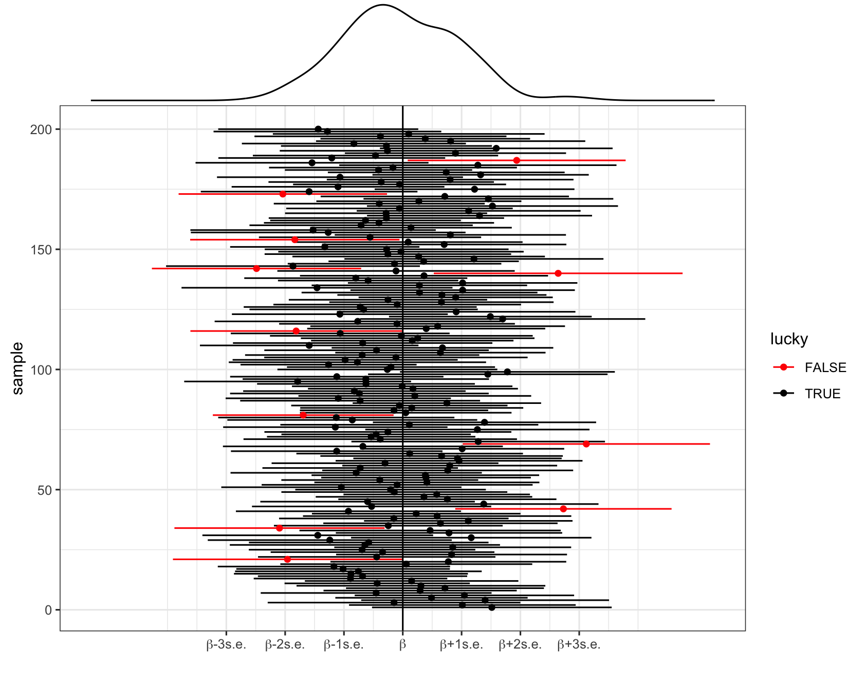
In pictures: 200 different 95% CIs for \beta calculated from 200 different samples. Each sample produces a different estimate \hat{\beta} (dot) hence a different 95% CI for \beta (horizontal line). Roughly 95% of these contain \beta (the black intervals) and roughly 5% do not (the red intervals).

Interpreting a CI

Let (a, b) represent the 95% CI for \beta.

Correct: We are 95% confident that \beta is between a and b.
Incorrect: There’s a 95% chance that \beta falls between a and b.
- Nope! \beta is either in there, or it isn’t. No probability involved.
- It is either in the interval or not, so the probability is 1 or 0.
Incorrect: There’s a 95% chance that sample estimate \hat{\beta} is between a and b.
- Nope! We have no uncertainty about \hat{\beta} – we know exactly what it is and it’s always in the interval by construction.

Exercises

Goals

Build up our confidence with confidence intervals (!) by starting with some familiar data and the simple linear regression setting.
Explore how to use CIs to assess the “significance” of our sample results.

Exercise 1: Standard errors

In the first set of exercises, we’ll explore daily bikeshare ridership. To begin, let’s explore the relationship of riders_total by windspeed (in mph):

E[riders_total | windspeed] = \beta_0 + \beta_1 windspeed

A sample estimate of this population model, obtained using our sample bikes data is below:

E[riders_total | windspeed] = \hat{\beta}_0 + \hat{\beta}_1 windspeed = 5621.15 - 87.51 windspeed

# Load packages and import data
library(tidyverse)
bikes <- read_csv("https://mac-stat.github.io/data/bikeshare.csv")

# Model the relationship
bikes_model_1 <- lm(riders_total ~ windspeed, data = bikes)
coef(summary(bikes_model_1))

# Visualize the relationship
bikes %>% 
  ggplot(aes(y = riders_total, x = windspeed)) + 
  geom_point() + 
  geom_smooth(method = "lm", se = FALSE)

Since \hat{\beta}_1 = -87.51, we estimate that the expected number of riders decreases by 87.51 for every 1mph increase in windspeed. Report and interpret SE(\hat{\beta}_1), the standard error of this estimate.
Considering context, units, and scale of our data (as illustrated in the plot), do you think this is a small, moderate, or large amount of error? (Mainly, do you think our slope estimate is pretty accurate or does the standard error make you skeptical?)

Exercise 2: Constructing & interpreting a CI

Continue to let \beta_1 be the “true” population windspeed coefficient, and \hat{\beta}_1 = -87.51 be our sample estimate of \beta_1.

\hat{\beta}_1 simply provides a point estimate, or our single best guess, of \beta_1. To also produce an interval estimate, use the 68-95-99.7 Rule to approximate a 95% CI for \beta_1.
We can calculate a more accurate CI by applying the confint() function to our model. Your approximation from Part a should be close!

confint(bikes_model_1, level = 0.95)

Interpreting the CI for \beta_1 in context requires that we can interpret \beta_1 itself! So how can we interpret \beta_1 (in general, without assuming a specific value for the unknown \beta_1)? Choose 1.

\beta_1 measures the expected number of riders on days with 0mph windspeed
\beta_1 measures the difference in the expected number of riders on days that have a lot of wind vs days that have little wind
\beta_1 measures the change in the expected number of riders for each additional 1mph in windspeed

Per the previous exercise: “We are 95% confident that \beta_1 is between -61.13 and -113.88”. Interpret this CI in context, drawing on your answer to Part a.

Exercise 3: Misinterpretations

For each of the following MISINTERPRETATIONS of a 95% confidence interval (a,b), explain why the statement is a misinterpretation.

Misinterpretation 1: “There is a 95% probability that the population parameter is within (a,b).”
Misinterpretation 2: “There is a 5% probability that the population parameter is not within (a,b).”
Misinterpretation 3: “There is a 95% chance that the sample estimate in (a,b).”

Exercise 4: Changing the confidence level

Our 95% CI for \beta_1 is (-113.88, -61.13). What would happen if we changed the confidence level?!

If we lower our confidence level from 95% to 68%, only 68% of samples would produce 68% CIs that cover \beta_1. Intuitively, would the 68% CI be narrower or wider than a 95% CI?
Use the 68-95-99.7 Rule to approximate the 68% CI for \beta_1.
What if we wanted to be VERY VERY confident that our CI covered \beta_1? Use the 68-95-99.7 Rule to approximate the 99.7% CI for \beta_1.
What if we wanted to be 100% confident that our CI covered \beta_1?!What do you think the CI would have to be?! (Use logic – the 69-95-99.7 Rule doesn’t help in this scenario.)
Check your answers to Parts b-d using confint(). (Your answers should be close but not exact.)

confint(bikes_model_1, level = 0.68)
confint(bikes_model_1, level = 0.997)
confint(bikes_model_1, level = 1)

Exercise 5: Trade-offs

Summarize the trade-offs in increasing confidence levels, say from 95% to 99.7%, for a CI of some population parameter \beta.

Choose the correct words for both statements. As confidence level increases…

the percent of CIs that cover \beta…increases / decreases / stays the same; and
the width of the CI…increases / decreases / stays the same.

Why is a very wide CI less useful than a narrower CI? For example, what if a pollster reported with 99.7% confidence that the support for “Candidate A” in an upcoming election is between 5% and 85%?
Practitioners typically use a 95% confidence level. Comment on why you think this is.

Exercise 6: Using CIs to test hypotheses

Recall our population model of interest:

E[time | windspeed] = \beta_0 + \beta_1 windspeed

A typical research question here might be whether, among the population of days (not just those in our sample), there’s a “significant” relationship between ridership and windspeed (i.e. \beta_1 \ne 0). Though our sample estimate suggested there’s a negative relationship (\hat{\beta}_1 = -87.51), there’s error in this estimate. So…does our sample still suggest a relationship after accounting for this potential error?!

The sample model is plotted below along with confidence bands that reflect its potential error. Based on this plot alone, what do you think? When accounting for the potential error in our sample model, do we have evidence of a “significant” relationship between ridership and windspeed?

bikes %>% 
  ggplot(aes(y = riders_total, x = windspeed)) + 
  geom_point() + 
  geom_smooth(method = "lm")

Recall that our 95% CI for \beta_1 was roughly (-113.88, -61.13). Using this CI alone, do we have evidence of a “significant” relationship between ridership and windspeed?
To answer Parts a and b, you had to make up some “rules” for using plots and CIs to evaluate the significance of \beta_1. In general, what were these rules?!

If (something about the plot), then our sample data provides evidence of a “significant” relationship between Y and X.
If (something about the CI), then our sample data provides evidence of a “significant” relationship between Y and X.

Your work above suggests that there’s a statistically significant association between ridership and windspeed. This merely suggests that an association exists (\beta_1 \ne 0). It does not necessarily mean that the magnitude of the association is meaningful, or practically significant, in context. Do you think that the association between riders_total and windspeed is also practically significant? Mainly, in the bikeshare context, is the magnitude of the association (a decrease between 61.13 and 113.88 riders per 1mph increase in windspeed) actually meaningful?

Extra Practice

The exercises below provide more practice with confidence intervals and other course concepts: visualizations, model building, logistic regression, causal diagrams, …. You will likely not get through all of these during class. That’s ok! Just remember to come back and practice after class.

Exercise 7: More practice

Research question: Is the relationship between wind speed (windspeed) (in miles per hour) and number of riders (riders_total) different across weekdays and weekends?

Construct and interpret a visualization that would address this question.
Fit a regression model that would address our research question. (Should it be a linear or a logistic regression model?) Interpret only the coefficient of interest.

mod_bikes <- ___

Construct an approximate 95% confidence interval (CI) for the coefficient of interest by hand using the 68-95-99.7 rule.
Compare your confidence interval to the one given by confint() which gives an exact confidence interval. (The columns give the lower and upper ends of the CI for each coefficient.)
Interpret the exact confidence interval in context.
Is zero in the interval? Do we have evidence for a real difference in the windspeed-riders relationship across weekends and weekdays?

# By hand (you fill in)


# Using confint()
confint(mod_bikes, level = 0.95)

Let’s see if these results agree when looking at adjusted R-squared.

Fit another regression model that does not have the coefficient of interest from your Part b model. Compare the adjusted R-squared values between this model and the Part b model. Explain your findings.

Exercise 8: Even more practice!

Research question: How different is holiday ridership from non-holidays, after accounting for confounding factors?

We believe that weather category (weather_cat), temperature (temp_actual), and wind speed (windspeed) confound the relationship of interest.

Draw a causal graph that shows the 5 variables of interest. Based on your graph do you believe that the 3 potential confounders are indeed confounders (and not mediators or colliders)?
Construct visualizations that allow you how each potential confounder relates to riders_total and to holiday.

Based on your Part a explorations, fit an appropriate regression model to answer our research question. Interpret only the coefficient of interest.

A note about scientific notation in R: Sometimes you may see numbers with the letter e in the middle. This is R’s way of expressing scientific notation. Whenever you see e, replace that with 10 to the power of .... So:

1.234e+02 is 1.234 x 10^2 = 123.4
1.234e-02 is 1.234 x 10^(-2) = 0.01234

Use confint() to construct a 95% confidence interval for the coefficient of interest.
Interpret this confidence interval in context.
Is zero in the interval? Do we have evidence for a real holiday effect on ridership?

Exercise 9: CIs with logistic regression

The Western Collaborative Group Study (WCGS) was designed in order to investigate a possible link between Type A behavior and coronary heart disease (CHD), and to develop a framework to select patients for intervention in order to decrease risk of CHD. The study contained 3154 cis men between the ages of 39 and 59 in California who had no history of CHD. They were enrolled in the study in 1960 and 1961, underwent a medical examination and covered their medical history, and they were re-examined annually for interim cardiovascular history.

A full codebook is available here. We will focus on the following variables:

chd: Presence (1) or absence (0) of CHD over followup (outcome)
tabp: Presence (1) or absence (0) of Type A behavior (main variable of interest)
age: Age at time of enrollment in the study (years)
sbp: Systolic blood pressure
dbp: Diastolic blood pressure
chol: Cholesterol (mg/dL)
ncigs: Number of cigarettes smoked per day
arcus: Presence (1) or absence (0) of arcus senilis (a colored ring around the cornea made up of lipids like cholesterol and believed to be a risk factor for CHD)
bmi: BMI = weight * 703 / height^2

Research question: Is there a causal effect of Type A/B personality on developing coronary heart disease?

wcgs <- read_csv("https://mac-stat.github.io/data/wcgs.csv")

We believe that the following variables are confounders of the relationship between Type A/B personality tabp and coronary heart disease (CHD): age + sbp + dbp + chol + ncigs + arcus + bmi.

Fit a regression model that would address our research question. (Should it be a linear or a logistic regression model?) Interpret only the coefficient of interest.

typea_mod <- ___

Construct a 95% confidence interval for the odds ratio of interest using the following code.
Interpret the confidence interval in context.
Is 1 contained in the interval? Why is 1 a relevant value to look for here?

(On your own time)

The data context in this exercise has a fraught history with the smoking industry. Read this article for some context about how the Type A personality came to be defined and studied. (One big takeaway: The smoking industry had a large incentive to find something to blame health problems on other than smoking!)

Reflection

How are you feeling about your ability to translate research questions into appropriate statistical investigations and addressing those questions using output from those investigations? What has gotten easier? What remains challenging?

Wrap-up

Finish and study the activity!
PS 6 posted and due next Monday

Solutions

Exercises

Exercise 1: Standard errors

Solution

# Load packages and import data
library(tidyverse)
bikes <- read_csv("https://mac-stat.github.io/data/bikeshare.csv")

# Model the relationship
bikes_model_1 <- lm(riders_total ~ windspeed, data = bikes)
coef(summary(bikes_model_1))

              Estimate Std. Error   t value      Pr(>|t|)
(Intercept) 5621.15288  185.06238 30.374368 1.361598e-131
windspeed    -87.50616   13.43266 -6.514433  1.359959e-10

# Visualize the relationship
bikes %>% 
  ggplot(aes(y = riders_total, x = windspeed)) + 
  geom_point() + 
  geom_smooth(method = "lm")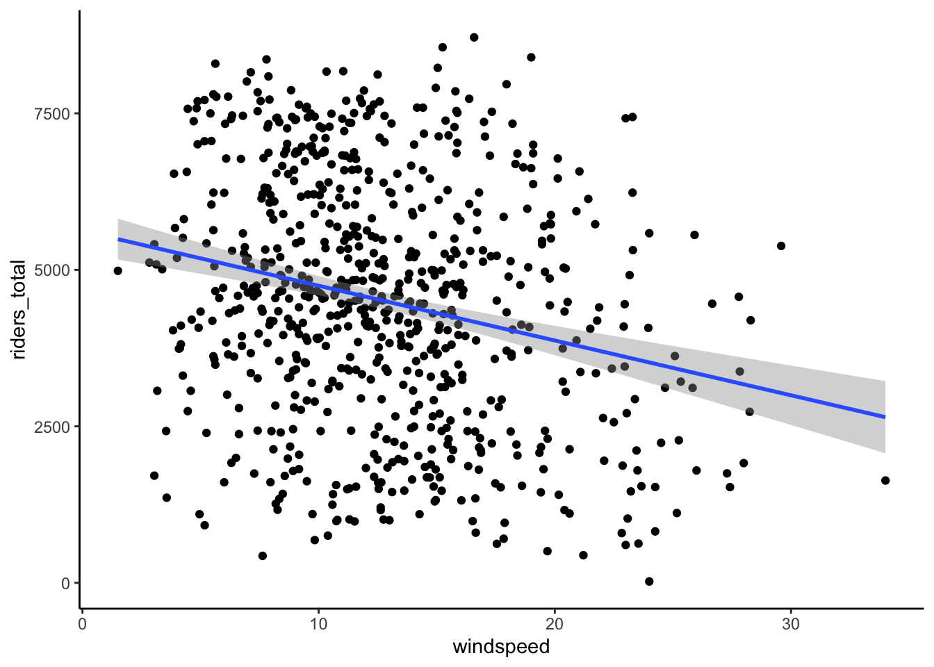

Though we estimate that the expected ridership decreases by 88 for every additional 1mph in windspeed, we expect that this estimate might be off by 13.4 riders/mph (that would be the typical error for a sample of this size).
This is a pretty small error – we think our slope estimate is pretty accurate. Relative to an estimate of 88 people / mph, being off by 13 people / mph is small both mathematically and contextually.

Exercise 2: Constructing & interpreting a CI

Solution

(-114.37, -60.65)

-87.51 - 2*13.43

[1] -114.37

-87.51 + 2*13.43

[1] -60.65

Pretty close!

confint(bikes_model_1, level = 0.95)

                2.5 %     97.5 %
(Intercept) 5257.8341 5984.47169
windspeed   -113.8775  -61.13485

\beta_1 measures the change in the expected number of riders for each additional 1mph in windspeed
We’re 95% confident that, for every additional 1mph in windspeed, the expected ridership decreases somewhere between 61 and 114 riders, on average.

Exercise 3: Misinterpretations

Solution

Misinterpretation 1: “There is a 95% probability that the population parameter is within (a,b).”
- Response: The population parameter is not random. It is either in the interval or not, so the probability is 1 or 0. The 95% means that 95% of random samples (that are representative of the population of interest) are expected to contain the true population parameter—“95% confidence” is describing confidence in the interval construction process.
Misinterpretation 2: “There is a 5% probability that the population parameter is not within (a,b).”
- Response: This is incorrect for the same reason as the first misinterpretation.
Misinterpretation 3: “There is a 95% chance that the sample estimate in (a,b).”
- Response: The sample estimate is always in the interval by construction.

Exercise 4: Changing the confidence level

Solution

Intuition.
(-100.94, -74.08)

-87.51 - 1*13.43

[1] -100.94

-87.51 + 1*13.43

[1] -74.08

(-127.8, -47.22)

-87.51 - 3*13.43

[1] -127.8

-87.51 + 3*13.43

[1] -47.22

Intuition.
.

confint(bikes_model_1, level = 0.68)

                 16 %       84 %
(Intercept) 5436.9905 5805.31524
windspeed   -100.8735  -74.13883

confint(bikes_model_1, level = 0.997)

               0.15 %    99.85 %
(Intercept) 5070.0833 6172.22246
windspeed   -127.5053  -47.50706

confint(bikes_model_1, level = 1)

             0 % 100 %
(Intercept) -Inf   Inf
windspeed   -Inf   Inf

Exercise 5: Trade-offs

Solution

As confidence level increases…

the percent of CIs that cover \beta…increases; and
the width of the CI…increases.

Narrower intervals are more precise. Wide intervals give us too many plausible values to be useful.
Partly this is just “tradition” – people use 95% because that’s what people have done for a long time! It’s more likely to cover the actual value than an interval with a lower confidence level (eg: 68%) but narrower, hence more useful / precise, than an interval with a higher confidence level (eg: 99.7%).

Exercise 6: Using CIs to test hypotheses

Solution

Yes! Any straight line that we can draw within the 95% confidence bands, i.e. the “range” of plausible population models, has a non-0 (specifically positive) slope.

bikes %>% 
  ggplot(aes(y = riders_total, x = windspeed)) + 
  geom_point() + 
  geom_smooth(method = "lm")

Yes! 0 is not in the interval (the whole CI is above 0), thus is not a plausible value. Thus even when accounting for the potential error in our sample estimate, it seems there’s an association between ridership and windspeed.

If a model with a slope of \beta_1 = 0 (a straight line) falls outside the confidence bands, then our sample data provides evidence of a “significant” relationship between Y and X.
If the CI for \beta_1 doesn’t include 0, then our sample data provides evidence of a “significant” relationship between Y and X.

Yes – considering the scale of ridership and windspeed, the estimated change in ridership with windspeed is meaningful in practice.

Exercise 7: More practice

Solution

Overall, windier days seem to have less riders (negative slope). The slope for weekends seems slightly steeper than for weekdays, but overall weekdays and weekends have similar slopes.

ggplot(bikes, aes(x = windspeed, y = riders_total, col = weekend)) + 
    geom_point(alpha = 0.2) +
    geom_smooth(method = "lm", se = FALSE) +
    theme_classic() +
    labs(x = "Windspeed (miles per hour)", y = "Total daily riders")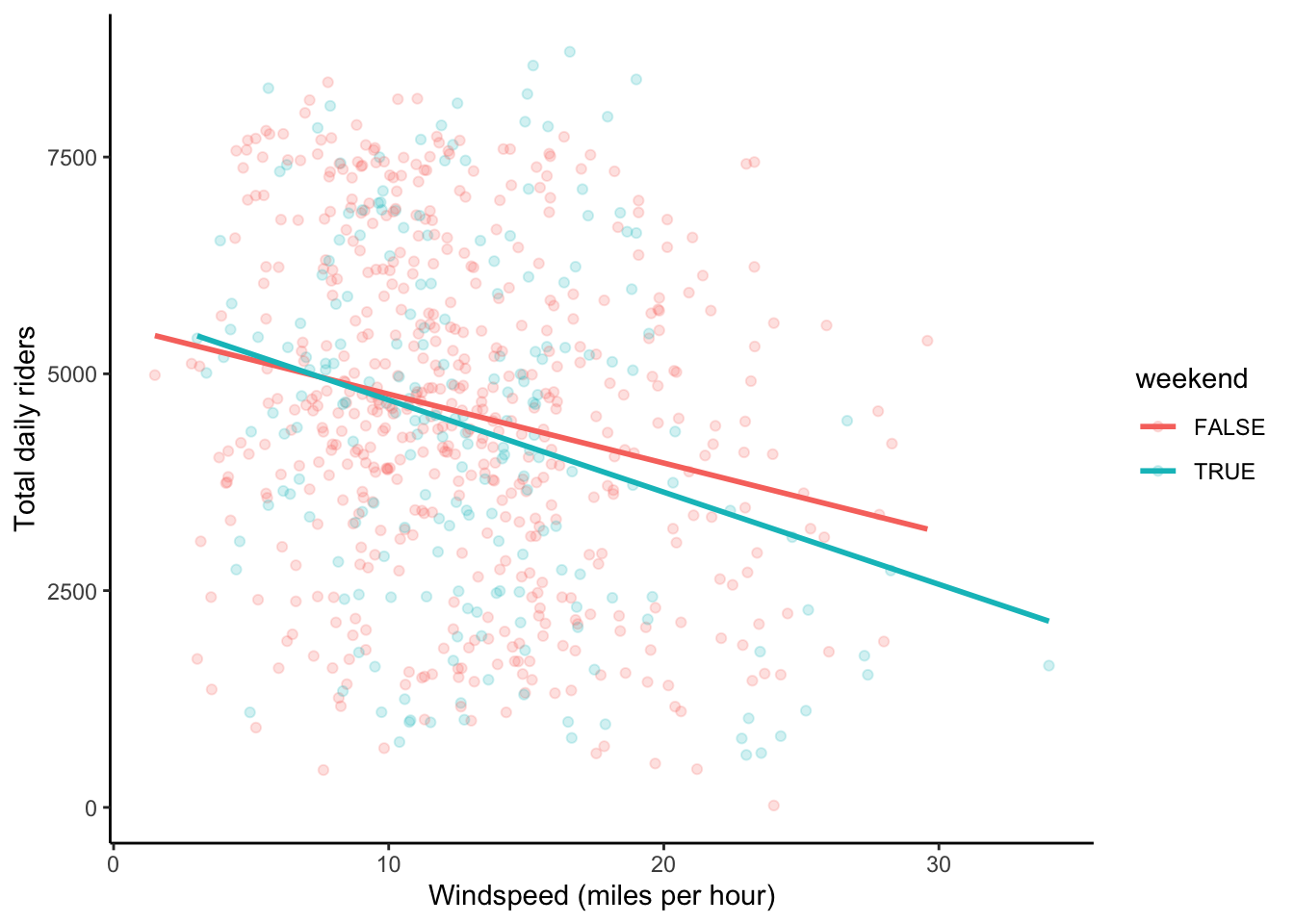

We need to fit a linear regression model (because outcome is quantitative) with an interaction term to answer this question. The interaction coefficient is of interest.

Interpretation of interaction coefficient: The average decrease in ridership associated with a 1 mph increase in wind speed is 26.82 rides/mph lower on weekends than for weekdays. Put another way, on weekdays, a 1 mph increase in wind speed is associated with a decrease of 79.47 riders. On weekends, that decrease is 106.29 riders.

mod_bikes <- lm(riders_total ~ windspeed*weekend, data = bikes)
summary(mod_bikes)


Call:
lm(formula = riders_total ~ windspeed * weekend, data = bikes)

Residuals:
    Min      1Q  Median      3Q     Max 
-4523.2 -1317.9   -46.9  1443.3  4715.7 

Coefficients:
                      Estimate Std. Error t value Pr(>|t|)    
(Intercept)            5560.31     219.07  25.382  < 2e-16 ***
windspeed               -79.47      15.97  -4.976 8.09e-07 ***
weekendTRUE             200.56     409.72   0.489    0.625    
windspeed:weekendTRUE   -26.82      29.56  -0.907    0.365    
---
Signif. codes:  0 '***' 0.001 '**' 0.01 '*' 0.05 '.' 0.1 ' ' 1

Residual standard error: 1885 on 727 degrees of freedom
Multiple R-squared:  0.05721,   Adjusted R-squared:  0.05332 
F-statistic:  14.7 on 3 and 727 DF,  p-value: 2.638e-09

Our manual calculation is pretty close to the CI given by confint().

Interpretation in context:

Preferred interpretation: It is plausible that the true population difference in the relationship between riders and wind speed comparing weekends to weekdays ranges from an average decrease of 84 riders/mph to an average increase of 31.21 riders/mph.

Not as preferred interpretation (but you’ll see this wording across disciplines): We are 95% confident that the difference in riders vs. wind speed slopes between weekends and weekdays is between -84 riders/mph to +31.21 riders/mph. (The instructors don’t like this interpretation as much because saying “95% confident” is rather vague. We are confident about the interval construction process across random samples, and this interpretation doesn’t make that clear.)

Zero is in the CI. This means that the difference in slopes could plausibly be zero. Therefore we do not have evidence for a real difference in the windspeed-riders relationship across weekends and weekdays.

# By hand
-26.82 - 2*29.56

[1] -85.94

-26.82 + 2*29.56

[1] 32.3

# By hand using 1.96, which is closer to the exact normal distribution quantile to use
-26.82 - 1.96*29.56

[1] -84.7576

-26.82 + 1.96*29.56

[1] 31.1176

# Using confint()
confint(mod_bikes, level = 0.95)

                           2.5 %     97.5 %
(Intercept)           5130.23243 5990.38552
windspeed             -110.81588  -48.11605
weekendTRUE           -603.82472 1004.93649
windspeed:weekendTRUE  -84.84192   31.21156

- The adjusted R-squared for the interaction model was 0.05332, compared to 0.05355 for the model without the interaction.
- Adding the interaction term actually decreased the adjusted R-squared, suggesting that it didn’t really improve the model.
- This agrees with what our CI interpretation: zero was a plausible value for the difference in slopes. If zero is a plausible value for the difference in slopes, allowing the slopes to be different in our model might not be necessary.

mod_bikes_noint <- lm(riders_total ~ windspeed+weekend, data = bikes)
summary(mod_bikes)


Call:
lm(formula = riders_total ~ windspeed * weekend, data = bikes)

Residuals:
    Min      1Q  Median      3Q     Max 
-4523.2 -1317.9   -46.9  1443.3  4715.7 

Coefficients:
                      Estimate Std. Error t value Pr(>|t|)    
(Intercept)            5560.31     219.07  25.382  < 2e-16 ***
windspeed               -79.47      15.97  -4.976 8.09e-07 ***
weekendTRUE             200.56     409.72   0.489    0.625    
windspeed:weekendTRUE   -26.82      29.56  -0.907    0.365    
---
Signif. codes:  0 '***' 0.001 '**' 0.01 '*' 0.05 '.' 0.1 ' ' 1

Residual standard error: 1885 on 727 degrees of freedom
Multiple R-squared:  0.05721,   Adjusted R-squared:  0.05332 
F-statistic:  14.7 on 3 and 727 DF,  p-value: 2.638e-09

summary(mod_bikes_noint)


Call:
lm(formula = riders_total ~ windspeed + weekend, data = bikes)

Residuals:
    Min      1Q  Median      3Q     Max 
-4563.0 -1323.1   -67.4  1445.2  4645.8 

Coefficients:
            Estimate Std. Error t value Pr(>|t|)    
(Intercept)  5659.76     189.64  29.845  < 2e-16 ***
windspeed     -87.29      13.44  -6.497 1.52e-10 ***
weekendTRUE  -143.87     154.07  -0.934    0.351    
---
Signif. codes:  0 '***' 0.001 '**' 0.01 '*' 0.05 '.' 0.1 ' ' 1

Residual standard error: 1885 on 728 degrees of freedom
Multiple R-squared:  0.05614,   Adjusted R-squared:  0.05355 
F-statistic: 21.65 on 2 and 728 DF,  p-value: 7.346e-10

Exercise 8: Even more practice!

Solution

Response: A causal graph might look like below (the double-headed arrows represent lines connecting the variables without a direction of causation). The variables that we’re considering putting in the model aren’t mediators or colliders. The visualizations support that weather_cat, temp_actual, and windspeed are causes of ridership, but only weather_cat and temp_actual seem to have noticeable differences between holidays and non-holidays.

dag <- dagitty::dagitty('
dag {
bb="0,0,1,1"
holiday [exposure,pos="0.123,0.550"]
riders_total [outcome,pos="0.668,0.545"]
temp_actual [pos="0.110,0.246"]
weather_cat [pos="0.439,0.260"]
windspeed [pos="0.276,0.157"]
holiday -> riders_total
holiday <-> temp_actual
holiday <-> weather_cat
holiday <-> windspeed
temp_actual -> riders_total
temp_actual -> weather_cat
weather_cat -> riders_total
windspeed -> riders_total
windspeed -> weather_cat
}
')
plot(dag)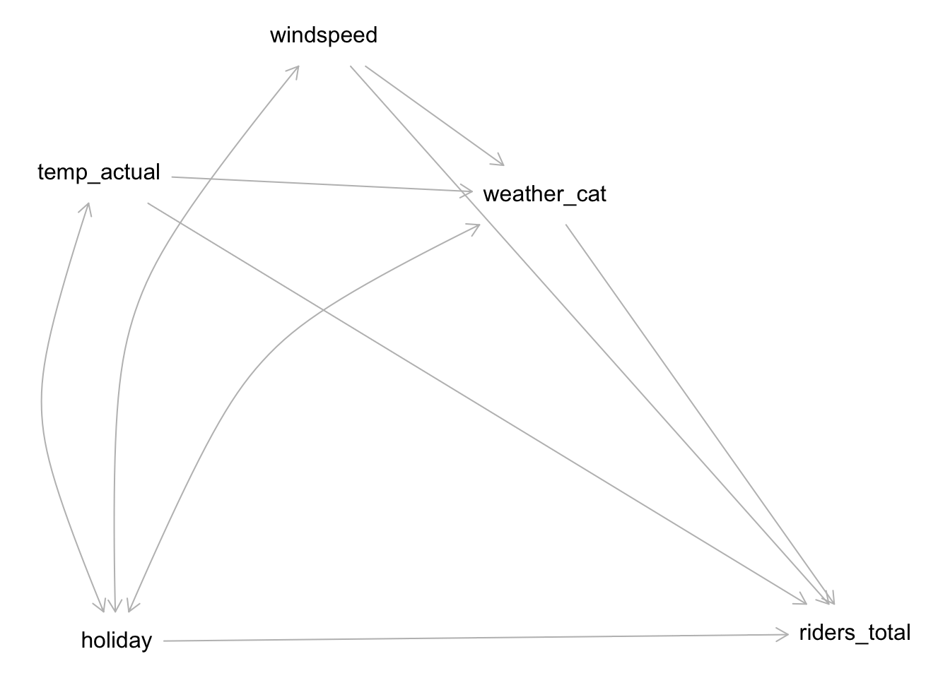

ggplot(bikes, aes(x = weather_cat, y = riders_total)) +
    geom_boxplot()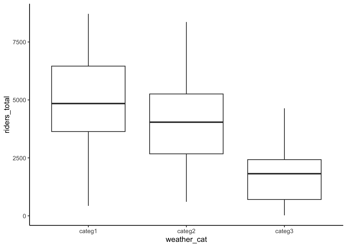

ggplot(bikes, aes(x = temp_actual, y = riders_total)) +
    geom_point() +
    geom_smooth()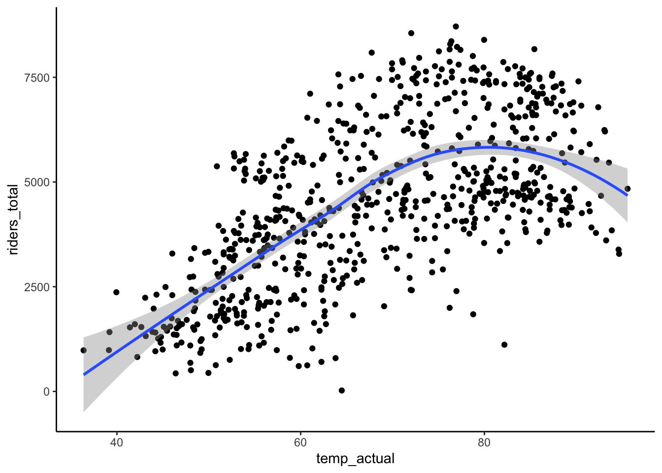

ggplot(bikes, aes(x = windspeed, y = riders_total)) +
    geom_point() +
    geom_smooth()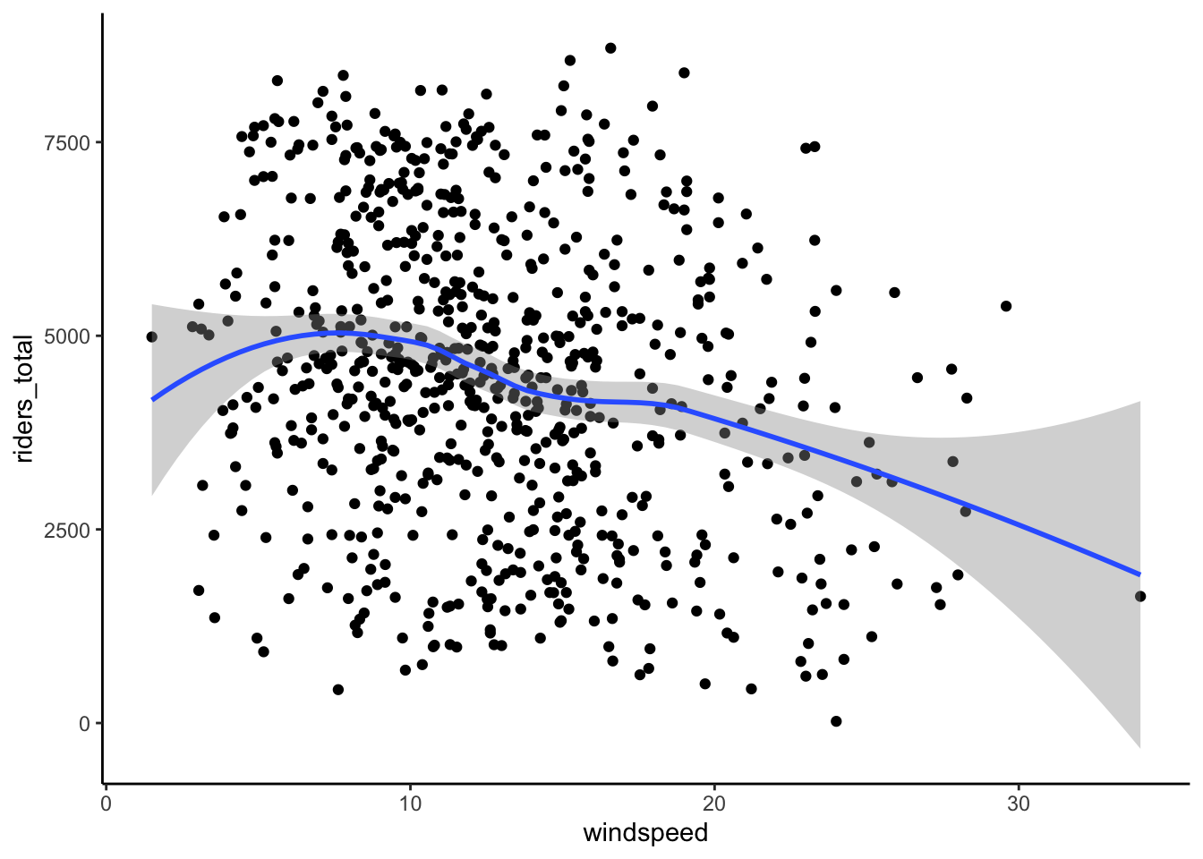

ggplot(bikes, aes(x = holiday, fill = weather_cat)) +
    geom_bar(position = "fill")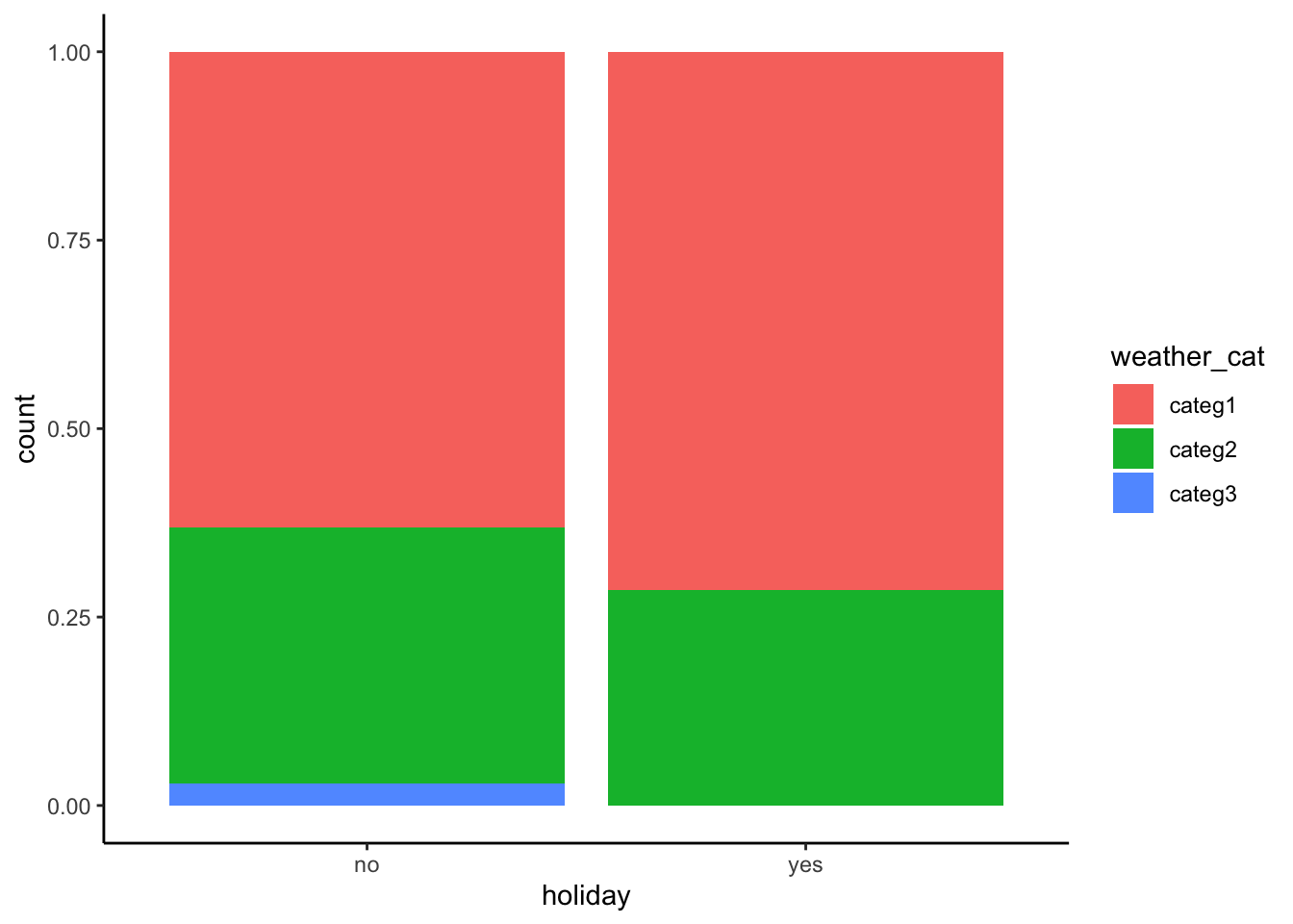

ggplot(bikes, aes(x = holiday, y = temp_actual)) +
    geom_boxplot()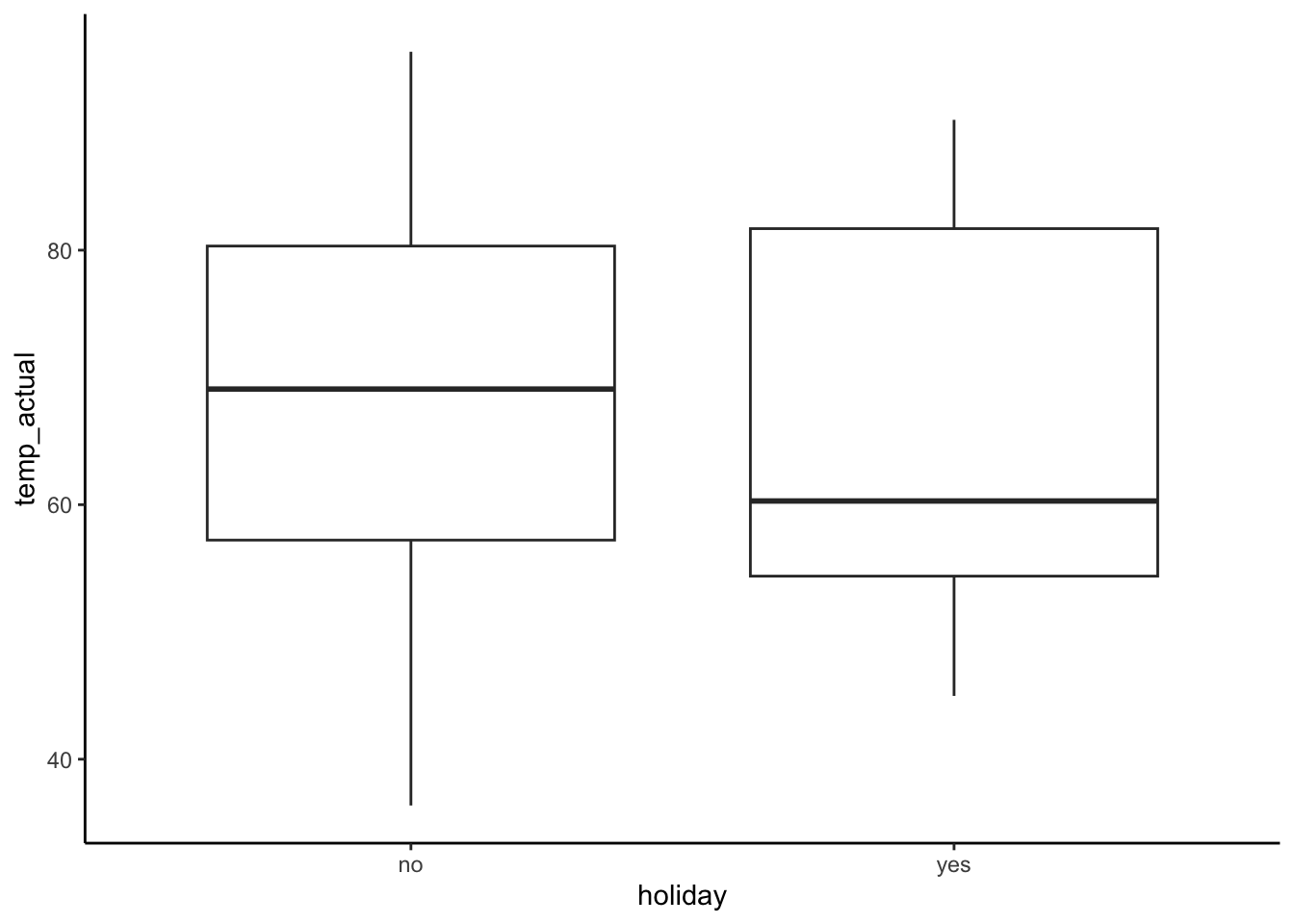

ggplot(bikes, aes(x = holiday, y = windspeed)) +
    geom_boxplot()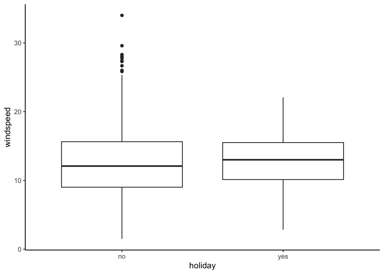

Response: Clear confounders from Part a include weather_cat and temp_actual. windspeed might be a precision variable because it don’t seem to be very different between holidays and non-holidays. We try models with just the confounders and with confounders+precision variable. Because temperature has a curved relationships with riders, we include a squared term.

The coefficient on holiday is of interest.

mod_bikes_smaller interpretation: Among days that have the same weather category and temperature, holidays have 731 fewer riders on average than non-holidays.

mod_bikes_larger interpretation: Among days that have the same weather category, temperature, and wind speed, holidays have 725 fewer riders on average than non-holidays.

bikes_new <- bikes %>% 
    mutate(
        temp_actual_squared = temp_actual^2
    )
mod_bikes_smaller <- lm(riders_total ~ holiday + weather_cat + temp_actual_squared, data = bikes_new)
mod_bikes_larger <- lm(riders_total ~ holiday + weather_cat + temp_actual_squared + windspeed, data = bikes_new)

summary(mod_bikes_smaller)


Call:
lm(formula = riders_total ~ holiday + weather_cat + temp_actual_squared, 
    data = bikes_new)

Residuals:
    Min      1Q  Median      3Q     Max 
-4225.5 -1200.7  -111.8  1057.8  3608.9 

Coefficients:
                      Estimate Std. Error t value Pr(>|t|)    
(Intercept)          1.872e+03  1.660e+02  11.280  < 2e-16 ***
holidayyes          -7.311e+02  3.263e+02  -2.240   0.0254 *  
weather_catcateg2   -5.708e+02  1.168e+02  -4.885 1.27e-06 ***
weather_catcateg3   -2.571e+03  3.297e+02  -7.799 2.18e-14 ***
temp_actual_squared  5.980e-01  2.973e-02  20.116  < 2e-16 ***
---
Signif. codes:  0 '***' 0.001 '**' 0.01 '*' 0.05 '.' 0.1 ' ' 1

Residual standard error: 1472 on 726 degrees of freedom
Multiple R-squared:  0.4257,    Adjusted R-squared:  0.4225 
F-statistic: 134.5 on 4 and 726 DF,  p-value: < 2.2e-16

summary(mod_bikes_larger)


Call:
lm(formula = riders_total ~ holiday + weather_cat + temp_actual_squared + 
    windspeed, data = bikes_new)

Residuals:
    Min      1Q  Median      3Q     Max 
-4050.0 -1109.6  -120.6  1068.0  3699.8 

Coefficients:
                      Estimate Std. Error t value Pr(>|t|)    
(Intercept)          2.577e+03  2.281e+02  11.294  < 2e-16 ***
holidayyes          -7.246e+02  3.222e+02  -2.249   0.0248 *  
weather_catcateg2   -5.924e+02  1.155e+02  -5.131 3.71e-07 ***
weather_catcateg3   -2.422e+03  3.272e+02  -7.403 3.70e-13 ***
temp_actual_squared  5.770e-01  2.973e-02  19.405  < 2e-16 ***
windspeed           -4.692e+01  1.057e+01  -4.439 1.05e-05 ***
---
Signif. codes:  0 '***' 0.001 '**' 0.01 '*' 0.05 '.' 0.1 ' ' 1

Residual standard error: 1454 on 725 degrees of freedom
Multiple R-squared:  0.4409,    Adjusted R-squared:  0.437 
F-statistic: 114.3 on 5 and 725 DF,  p-value: < 2.2e-16

Response: We’ll focus on the CI from mod_bikes_smaller since the CI from mod_bikes_larger is pretty similar.

Interpretation in context:

Preferred interpretation: It is plausible that the true population difference in average holiday ridership vs. average non-holiday ridership is from 1371.8 to 90.5 fewer rides on holidays (among days of the same weather category and temperature).

Not as preferred interpretation: We are 95% confident that the population difference in holiday vs non-holiday ridership is between -1371.8 to -90.4532521.

Zero is not in the CI which means that the difference between holidays and non-holidays (among days of the same weather category and temperature) is not plausibly zero. We do have evidence for a true holiday effect.

confint(mod_bikes_smaller, level = 0.95)

                            2.5 %        97.5 %
(Intercept)          1546.3798240  2198.1156306
holidayyes          -1371.8105006   -90.4532521
weather_catcateg2    -800.1540608  -341.3738083
weather_catcateg3   -3218.3124545 -1923.8150951
temp_actual_squared     0.5396379     0.6563642

confint(mod_bikes_larger, level = 0.95)

                           2.5 %        97.5 %
(Intercept)          2128.817226  3024.6176444
holidayyes          -1357.222742   -92.0407887
weather_catcateg2    -819.136285  -365.7464372
weather_catcateg3   -3064.923766 -1780.0402827
temp_actual_squared     0.518586     0.6353312
windspeed             -67.677428   -26.1684414

Exercise 9: CIs with logistic regression

Solution

wcgs <- read_csv("https://mac-stat.github.io/data/wcgs.csv")

Response: We need to fit a logistic regression model because the chd outcome is binary. We include tabp as the main predictor of interest and all of the other confounding variables. We need to exponentiate the coefficient so that we’re interpreting on the odds scale rather than the log odds scale.

Interpretation of exp(tabp): Among men of the same age, systolic and diastolic blood pressure, cholesterol levels, smoking habits, history of arcus sinilis, and BMI, those with Type A personality have 1.95 times the odds of CHD than those without Type A personality.

typea_mod <- glm(chd ~ tabp + age + sbp + dbp + chol + ncigs + arcus + bmi, data = wcgs, family = "binomial")
summary(typea_mod)


Call:
glm(formula = chd ~ tabp + age + sbp + dbp + chol + ncigs + arcus + 
    bmi, family = "binomial", data = wcgs)

Coefficients:
              Estimate Std. Error z value Pr(>|z|)    
(Intercept) -1.225e+01  9.898e-01 -12.378  < 2e-16 ***
tabp         6.670e-01  1.458e-01   4.576 4.74e-06 ***
age          5.897e-02  1.230e-02   4.794 1.64e-06 ***
sbp          1.824e-02  6.408e-03   2.846  0.00443 ** 
dbp         -5.797e-04  1.086e-02  -0.053  0.95743    
chol         1.045e-02  1.519e-03   6.879 6.04e-12 ***
ncigs        2.131e-02  4.287e-03   4.971 6.67e-07 ***
arcus        2.219e-01  1.436e-01   1.545  0.12238    
bmi          5.841e-02  2.714e-02   2.152  0.03141 *  
---
Signif. codes:  0 '***' 0.001 '**' 0.01 '*' 0.05 '.' 0.1 ' ' 1

(Dispersion parameter for binomial family taken to be 1)

    Null deviance: 1769.2  on 3139  degrees of freedom
Residual deviance: 1572.6  on 3131  degrees of freedom
  (14 observations deleted due to missingness)
AIC: 1590.6

Number of Fisher Scoring iterations: 6

coef(typea_mod)

  (Intercept)          tabp           age           sbp           dbp 
-1.225217e+01  6.670497e-01  5.897199e-02  1.823715e-02 -5.797328e-04 
         chol         ncigs         arcus           bmi 
 1.045016e-02  2.131124e-02  2.218750e-01  5.840654e-02

exp(coef(typea_mod))

 (Intercept)         tabp          age          sbp          dbp         chol 
4.774751e-06 1.948480e+00 1.060746e+00 1.018404e+00 9.994204e-01 1.010505e+00 
       ncigs        arcus          bmi 
1.021540e+00 1.248415e+00 1.060146e+00

Response:

Interpretation in context:

Preferred interpretation: Among men of the same age, systolic and diastolic blood pressure, cholesterol levels, smoking habits, history of arcus sinilis, and BMI, it is plausible that those with Type A personality have 1.47 to 2.60 times the odds of CHD than those without Type A personality.

1 is not in the CI. 1 is a relevant value to consider for ratios because if the odds ratio is 1, then the (adjusted) odds of CHD is the same in those with Type A and Type B personality. There seems to be a positive relationship between Type A personality and CHD in this study.

confint(typea_mod, level = 0.95) %>% exp()

                   2.5 %       97.5 %
(Intercept) 6.706495e-07 3.257156e-05
tabp        1.469222e+00 2.603660e+00
age         1.035479e+00 1.086677e+00
sbp         1.005561e+00 1.031169e+00
dbp         9.783446e-01 1.020911e+00
chol        1.007521e+00 1.013538e+00
ncigs       1.012938e+00 1.030126e+00
arcus       9.399791e-01 1.651412e+00
bmi         1.004943e+00 1.117811e+00