Connecting context with our understanding of statistical concepts, we’re prepared to think critically about our hypothesis testing result as well as those of others!
ImportantLearning goals
By the end of this lesson, you should be able to:
Differentiate between more and less accurate interpretations of p-values
Understand Type I vs Type II error, as well as statistical power
Explain the difference between practical and statistical significance
Explain how multiple testing impacts the conduct and interpretation of statistical research
ImportantAdditional resources
No new readings or videos for today.
Conclusions from Hypothesis Testing
Test Statistic
P-Value
Conclusion
|z_{obs}| > 3
p-value < 0.003
Data very incompatible with H_0
2 < |z_{obs}| < 3
0.003 < p-value < 0.05
Data moderately incompatible with H_0
1 < |z_{obs}| < 2
0.05 < p-value < 0.32
Data somewhat compatible with H_0
| z_{obs} | < 1
p-value > 0.32
Data compatible with H_0
P-value: the probability of getting a test statistic as large or larger than observed, assuming the null hypothesis is true.
How large of a test statistic (or small of a p-value) do we need to reject H_0?
Significance Level: a p-value threshold, determined prior to data collection & analysis, that defines “incompatibility” between the observed data and the null hypothesis.
Reject H_0 if p-value < significance level.
If we use a significance level of 0.01,
p-value = 0.001: Reject the Null Hypothesis
p-value = 0.046: Fail to Reject the Null Hypothesis
p-value = 0.16: Fail to Reject the Null Hypothesis
If we use a significance level of 0.05,
p-value = 0.001: Reject the Null Hypothesis
p-value = 0.046: Reject the Null Hypothesis
p-value = 0.16: Fail to Reject the Null Hypothesis
If we use a significance level of 0.1,
p-value = 0.001: Reject the Null Hypothesis
p-value = 0.046: Reject the Null Hypothesis
p-value = 0.16: Fail to Reject the Null Hypothesis
But we could be wrong?! In 2 different ways…
Type 1 Error: reject H_0 when H_0 is actually true
Consequences: Headlines such as “coffee causes cancer” when in fact it doesn’t
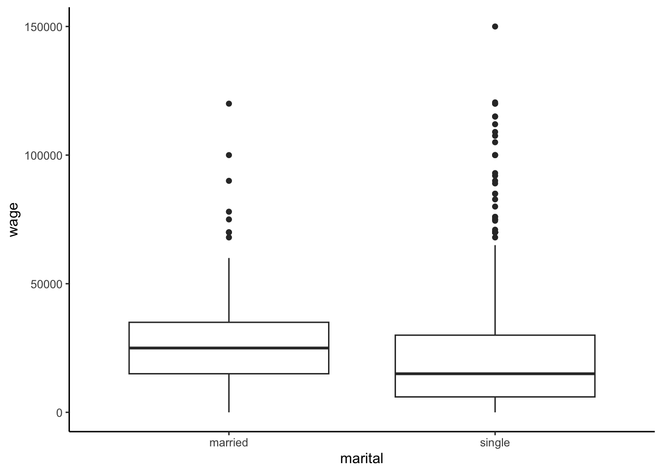
We estimate that the expected / average wage for single workers is $6596.13 below that of married workers.
We expect that this estimate might be off by / have an error of $1817.41.
We’re 95% confident that, in the broader labor force, the average wage among single workers is somewhere between $3030.63 and $10161.64 lower than that of married workers. Thus we have statistically significant evidence that wage is associated with marital status (a difference of $0 isn’t in this interval, hence isn’t a plausible value).
Example 1: Hypothesis test review
Consider the following hypotheses:
H_0: \beta_1 = 0 (wage is not associated with marital status)
H_a: \beta_1 \ne 0 (wage is associated with marital status)
Evaluate these hypotheses using a 0.05 significance level.
Be sure to state a clear conclusion, and support that conclusion with appropriate evidence.
Example 2: p-value
The p-value for the above test was 0.0003 (which is very small!). How can we interpret this p-value?
Given our sample data, it’s very unlikely that wages are associated with marital status (i.e. that H_a is true). P(H_a | data) = \text{prob of $H_a$ being true given our data}
Given our sample data, it’s very unlikely that wages and marital status are unrelated (i.e. that H_0 is true). P(H_0 | data) = \text{prob of $H_0$ being true given our data}
If in fact there were no relationship between wages and marital status in the broader labor force (i.e. H_0 were true), it’s unlikely that we’d have observed such a big wage gap between single and married workers “by chance”. P(data | H_0) = \text{prob of observing our data given $H_0$ is true}
Example 3: Just some considerations
Hypothesis tests are a powerful tool, but need to be considered carefully!
Causal misinterpretations. The above results do not establish a causal association between wage and marital status, i.e. that being single leads to lower wages. Why?
Statistical vs practical significance. We observed a statistically significant association between wages and marital status. BUT statistical significance merely indicates evidence that an association between wages and marital status exists (it’s non-0). Consider an important follow-up: is the magnitude or size of this association (a $3,030.63–$10,161.64 wage gap) practically significant / contextually meaningful?
confint(wage_model_1)
Type I & Type II errors. Our test might have led us to an incorrect conclusion, not because we did anything wrong, but because we got unlucky data! Check out the errors below. What type of error might we have made in our conclusion about wages and marital status?
Conclusion
H_0 actually true
H_0 actually false
fail to reject H_0
correct!
Type II error (false negative)
reject H_0
Type I error (false positive)
correct!
Example 4: Type I & Type II error rate
Type I and Type II error rates measure the chance that we end up making one of these errors. These can be expressed as conditional probabilities:
Type I Error (false positive) rate
P(reject H_0 | H_0 actually true)
P(conclude an effect does exist when it actually doesn’t)
Type II Error (false negative) rate
P(fail to reject H_0 | H_0 actually false)
P(conclude an effect doesn’t exist when it actually does)
Type II error rates depend upon various factors, that we only have some control over (e.g. actual effect size and sample size). However, we do have control Type I error rate. How?
Exercises
Goal
Practice and consider some nuances to be aware of in hypothesis testing.
Exercise 1: Conceptual understanding
Suppose that you and a friend are in two different sections (each with the same number of students) of the same class. On your respective midterm exams, you each obtained 85%, and the class average in both of your classes was 80%. Could one of you or your friend still be considered further above the class average than the other? Briefly explain.
Now suppose that your section’s test scores were more tightly packed around 80%: maybe the standard deviation of your section’s scores was 2.5, whereas the standard deviation of your friend’s section’s scores was 5. Which of you or your friend was further above the class average? Explain/justify your answer.
Broadly speaking, does a p-value measure the chance of a hypothesis being true, or, the chance of the data having occurred?
Why can’t a p-value measure the other quantity that you didn’t choose in Part c?
Explain in words why, in calculating a p-value, we need to assume that the null hypothesis is true.
Suppose that a hypothesis test yields a p-value of 1e-6 (1\times 10^{-6}). What can you tell about the magnitude of the effect or the uncertainty of the effect from this p-value? (i.e., What can you tell about the coefficient estimate or the standard error?)
Exercise 2: Statistical vs. practical significance
Music researchers compiled information on 16,216 Spotify songs. They examined the relationship between a song’s genre (latin vs. not latin) and song duration in seconds. Their modeling code and output is below:
Based on their below plot of duration by latin_genre, does song duration appear to be associated with genre?
spotify %>%ggplot(aes(y = duration, x = latin_genre)) +geom_boxplot()
Check out a model of this relationship and interpret the latin_genreTRUE coefficient. In the context of song listening, is this a meaningful effect size?
Report and interpret the p-value for the latin_genreTRUE coefficient.
Use the p-value to make a yes/no decision about the evidence for a relationship between genre and song duration.
This exercise highlights the difference between statistical significance and practical significance. Explain why this happened. That is, when might we observe statistically significant results that aren’t practically significant? (Hence when should we be especially cautious about interpreting the results of a hypothesis test?)
Exercise 3: Full model context
When interpreting hypothesis tests, we must be consider the full model context – what else is / is not in our model? Consider our question about a wage gap and marital status. Compare and contrast our conclusions from the maritalsingle coefficient in the 2 models below, one of which controls for age, a potential confounder.
IMPORTANT: These results are not contradictory! Rather, together they provide a more complete picture about the relationship of interest.
wage_model_1 <-lm(wage ~ marital, data = cps)coef(summary(wage_model_1))wage_model_2 <-lm(wage ~ marital + age, data = cps)coef(summary(wage_model_2))
Exercise 4: Power
Recall: Via our chosen significance level (typically 0.05), we control the Type I error (aka false positive) rate:
P(Type I error) = P(reject H_0 | H_0 is actually true) = 0.05
We have less control over the Type II error (aka false negative) rate:
P(Type II error) = P(fail to reject H_0 | H_0 actually false) = ???
An important related concept is that of statistical power, the true positive rate. Specifically, power is the probability of (correctly!) rejecting H_0 when H_0 is actually false:
power = P(reject H_0 | H_0 actually false) = 1 - P(Type II error)
Less formally, statistical power is the probability of detecting a relationship when there truly is a relationship. Thus power is a good thing!! We want it to be as high as possible!! Mainly, if an effect exists, we want there to be a high chance that we detect it.
Unfortunately, we can’t control power. It’s influenced by various factors. Navigate to this page to check out an interactive visualization of the factors that influence statistical power.
Under “Settings”, next to the “Solve for?” text, click “Power”. You will vary the 3 different parameters (significance level, sample size, and effect size) one at a time to understand how these factors affect power.
Some context behind this interactive visualization:
Visualization is based on a one sample Z-test:
This is a test for whether the true population mean equals a particular value. (e.g., true mean = 30)
The effect size slider is measured with a metric called Cohen’s d:
Cohen’s d = magnitude of effect/standard deviation of response variable
Here: how far is the true mean from the null value in units of SD?
e.g., If the null value is 30, true mean is 40, and the true population SD of the quantity is 5, the Cohen’s d effect size is (40-30)/5 = 2.
What is your intuition about how changing the significance level will change power? Check your intuition with the visualization and explain why this happens.
Could I replicate these results if I got a different sample than them?
What was their motivation?
How did they measure their variables? Might their results have changed if they used different measurements?
Check out an interactive tool that helps you explore these ideas: https://stats.andrewheiss.com/hack-your-way/ Use this tool to “prove” 2 different claims. For both, be sure to indicate what response variable (eg: Unemployment rate) and data (eg: senators) you used:
the economy is significantly better when Republicans are in power
the economy is significantly better when Democrats are in power
Exercise 6: Multiple testing
In the previous exercise, parts b and c illustrate the dangers of multiple testing: the more things we test, the more likely something will appear to be “significant” just by chance (even if it’s not). Thus fishing around for significance can lead to misleading conclusions.
Let’s consider some math. Using a 0.05 significance level, if we perform 1 test the probability of getting a Type I error is 0.05. If we perform 2 tests (with H_0 being true in each case), the probability of getting at least 1 Type I error is:
Pr(at least one Type I error) = 1 - P(no Type I errors) = 1 - (1 - 0.05)^2 = 0.0975
1- (1-0.05)^2
This is called the overall or family-wise Type I error rate. If we perform 3 tests (with H_0 being true in each case), the probability of getting at least 1 Type I error is:
Pr(at least one Type I error) = 1 - P(no Type I errors) = 1 - (1 - 0.05)^3 = 0.1426
1- (1-0.05)^3
Calculate the probability of getting at least 1 Type I error if we perform 20 tests (with H_0 being true in each case). This is how many tests were completed in the jelly bean example!
What’s the takeaway from part a?
If you are a Bio major, read on: To counter the phenomenon above, one solution when doing multiple testing is to inflate the observed p-value from each test. For example, the Bonferroni method penalizes for testing ‘too many’ hypotheses by artificially inflating the p-value:
Bonferroni-adjusted p-value = observed p-value * total # of tests
Equivalently, we artificially deflate the significance level:
Bonferroni-adjusted significance level = 0.05 / total # of tests
For example, if we do 20 tests at the 0.05 level, we reject each H_0 if its p-value is less than 0.0025 (i.e. 0.05/20). This makes it tougher to reject H_0, thus to make a Type I error. BUT what are the trade-offs? NOTE: There are less conservative approaches out there! Bonferroni is just easy to use.
Wrap Up
Finish and study the activity!
PS 7 due tonight
Project Milestone 2 due Friday night
PS 8 due next Monday
Check out the course schedule for other upcoming due dates (last CP coming up!).
Reminders:
Remember the important basics: complete activities, ask for help, study on a regular basis, start assignments early.
If you miss class on a project day, it’s your responsibility to communicate with your group, find out what you missed, and make equivalent contributions outside of class. If missing class on project days becomes a pattern, it will impact your project grade.
Your final project grade will reflect your individual engagement and contributions to the project. You are not expected to be perfect. Rather, you should put effort, attention, and reflection into the following areas:
communication
contributing to group discussions
including all other group members in discussion
creating a space where others felt comfortable sharing ideas and mistakes
communicating with your group outside class
report contributions
contributing to the content / analysis in the report
contributing to the writing of the report
contributing to the editing of the report
Solutions
Exercises
Exercise 1: Conceptual understanding
Solution
Yes! How well you do relative to the rest of the class depends on both the class average AND the variability of scores in each section. In this case, if your section was more variable, 85% wouldn’t be as far above the class average than in your friend’s section.
In this case, we could note that your score of 85 was 2 standard deviations above the class average (85-80)/2.5 = 2, whereas your friend’s score was only one standard devation above the class average (85-80)/5 = 1. Here, your score would be considered more extreme, and therefore further above the class average than your friend’s score.
the chance of the data having occurred?
Broadly speaking, the latter is more correct. By definition, a p-value measures the probability that an observation (as or more extreme that what did observe) would occur over repeated sampling under the null hypothesis (if the null hypothesis were true). This does NOT measure the chance of a hypothesis being true, but rather, tries to make a statement about the null hypothesis through indirect means.
In order to make probabilistic statements about repeatedly sampled measures (as p-values do), we need to first be able to define a probability distribution. The null hypothesis tells us where this probability distribution is centered. As a concrete example, we can’t answer questions like “what is the chance we observed this data?” without making some assumption about what the underlying truth is, or sometimes, where the truth is unlikely to be. For example, if we observe a regression coefficient of 2.3, we don’t know if this is likely or not. We can say, however, how likely it is we would observe 2.3 if the true population coefficient were 2 compared to if the true population coefficient were 0.5.
A p-value tells us nothing about the coefficient estimate or the standard error because it only tells us about the test statistic. A small p-value only indicates that the test statistic is large. A large test statistic could have come about from a large effect (large coefficient) or from a small coefficient with a very small standard error. This is why reporting a confidence interval is more informative than only reporting a p-value. We get a sense of both the magnitude of the estimate and the amount of uncertainty with a CI, and with just a p-value, we don’t know either.
Exercise 2: Statistical vs. practical significance
NO! The distribution of duration is nearly indistinguishable between the 2 genres.
spotify %>%ggplot(aes(y = duration, x = latin_genre)) +geom_boxplot()
On average, latin genre songs tend to be 1.56 seconds longer than non-latin songs. This is NOT a meaningful difference – 1.56 seconds in a song is really short.
If there were truly no difference in the duration of latin vs non-latin songs (in the broader population of songs), there’s only a 3.6% chance that we would have obtained a sample in which the observed difference was so large relative to the amount of uncertainty in the estimate (the standard error).
We have statistically significant evidence that latin genre songs tend to be longer than non-latin songs.
Our large sample size of over 16,000 songs is relevant. The more data we have, the smaller our standard errors. (Recall that standard errors are inversely proportionaly to the square root of sample size: std error = c/\sqrt{n}, where c is a constant from complicated formulas.) Larger sample sizes lead to narrower CIs, larger test staistics, and smaller p-values. With large sample sizes, it is easier to find statistically significant results even when the results aren’t practically significant.
Exercise 3: Full model context
Solution
Though there’s an overall significant association between wage and marital status (per wage_model_1), that association is not significant when controlling for age (per wage_model_2).
wage_model_1 <-lm(wage ~ marital, data = cps)coef(summary(wage_model_1))
               Estimate Std. Error   t value     Pr(>|t|)
(Intercept)   27399.471   1714.496 15.981066 1.849857e-52
maritalsingle -6596.133   1817.411 -3.629412 2.955178e-04
wage_model_2 <-lm(wage ~ marital + age, data = cps)coef(summary(wage_model_2))
                Estimate Std. Error    t value     Pr(>|t|)
(Intercept)   -53547.003  5719.1332 -9.3627830 3.484809e-20
maritalsingle  -1456.015  1714.3082 -0.8493312 3.958595e-01
age             3483.197   236.4797 14.7293716 2.099717e-45
Exercise 4: Power
Solution
Overall notes about the power investigations:
Because power is the probability of correctly rejecting the null hypothesis (rejecting the null when the alternative hypothesis is true), parameter changes that increase the frequency of rejecting the null hypothesis will increase power. Keep this in mind as you work through. Visually, power corresponds to the light blue area under the distribution on the right. The distribution on the left is our familiar sampling distribution of the test statistic (here called Z_{\text{crit}}) under the null. The distribution on the right is very closely related but is the sampling distribution of the test statistics under the alternative hypothesis (which is why the H_A label is above it). Power corresponds to the light blue area under the H_A distribution because this area actually corresponds to the test statistics for which we would reject the null. The area represents the probability that we would obtain such test statistics if indeed the alternative were true. That is, the area represents the percentage of samples that would generate test statistics large enough to reject the null (if the alternative hypothesis were true).
Effect of significance level:
If the significance level increases, there is a “less stringent” threshold for rejecting the null (p-value only has to be less than some higher threshold). Increasing the significance level will result in more frequent rejections of the null, and thus higher power (but at the price of a higher type 1 error rate).
Effect of sample size:
If sample size increases, power should increase because higher sample size will decrease standard error, which will increase the test statistic, which more likely leads to rejecting the null.
Effect of effect size:
If the magnitude of the effect (numerator of Cohen’s d) increases, power should increase because it is easier (we are more likely) to detect large effects. It is harder (we are less likely) to detect very small effects.
If the variability of the response variable decreases (denominator of Cohen’s d), power should increase because any “signal” from our predictors being picked up by our coefficient estimates will rise far enough above the “noise” in the small variability of the response. The variability of the response variable also contributes to the standard error for the coefficient. With low variability of the response, we will have lower standard errors because there will be lower spread in the estimates across samples. And with lower standard errors, test statistics should increase, resulting in greater frequency of rejecting the null.
A large effect magnitude and small variability in the response result in a large effect size, and increasing effect size results in higher power.
Exercise 5: Ethical considerations
Solution
The comic is an illustration of something called the file drawer phenomenon. There is a culture that has arisen when using hypothesis testing in statistical analysis to only appreciate rejections of the null hypothesis as meaningful results. Any results for which investigators were not able to reject the null were filed away, never to be reported. Investigators would keep trying until their p-values were lower than the significance level.
There are serious ethical considerations behind this phenomenon. Who ever said that rejecting the null hypothesis was the only way to get meaningful scientific results? There is immense benefit in knowing when there are no effects / no relationships. A very important public health example of this is the relationships between vaccination and autism risk in children. Time and time again, studies have not been able to detect any causal relationship. What would our society look like if those “null” results had been filed away, never to be reported?
The idea here is that many, many hypothesis tests are being conducted, which is an idea called multiple testing. As more and more tests are being conducted, there is a higher and higher overall chance that the null hypothesis will be rejected - because we’re just trying so many times. If the null hypothesis is in fact true, testing more and more times is going to increase the probability of making at least one type 1 error.
In this comic, we would likely be inclined to believe that the null hypothesis is true (no true association between jelly bean eating and acne). But the sheer number of times that this hypothesis was tested (20 times) means that the scientists ended up finding an association just by chance. That is, the association found for green jelly beans was quite likely a type 1 error. And in fact one null hypothesis rejection among 20 tests is exactly a 5% error rate - in other words, exactly the number of null hypothesis rejections we would expect to make if indeed the null were true (exactly the expected number of type 1 errors).
Exercise 6: Multiple testing
Solution
1- (1-0.05)^20
[1] 0.6415141
The more tests we do, the more likely we are to make a Type I error (false positive).
This makes it tough to establish statistical significance (the p-value would have to be very, very low). Thus this might increase the Type II error rate, i.e. we might make more false negatives.